RAID Penalty Calculator
Estimate RAID read IOPS, write penalty, blended workload capacity, usable storage, and rebuild reserve for home NAS, virtualization, media, and backup arrays.
RAID I/O estimate
| RAID level | Minimum disks | Usable capacity formula | Random write penalty | Good fit |
|---|---|---|---|---|
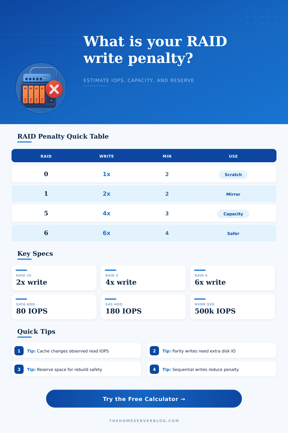
| RAID 0 | 2 | N disks | 1x | Temporary scratch where failure is acceptable |
| RAID 1 | 2 | 1 disk per mirror pair | 2x | Small boot volumes and two-bay NAS systems |
| RAID 5 | 3 | N - 1 disks | 4x | Read-heavy capacity arrays with modest writes |
| RAID 6 | 4 | N - 2 disks | 6x | Larger HDD pools that need dual parity |
| RAID 10 | 4 | N / 2 disks | 2x | VMs, databases, and mixed random I/O |
| RAID 50 | 6 | N - number of RAID 5 sets | 4x | Capacity plus more spindles than one RAID 5 set |
| RAID 60 | 8 | N - 2 per RAID 6 set | 6x | Large archival pools with dual parity per set |
| Disk class | Typical random IOPS | Latency tendency | Queue behavior | Calculator use |
|---|---|---|---|---|
| 5.4K SATA HDD | 55-75 | High | Needs gentle queues | Cold media, backups, light NAS |
| 7.2K SATA HDD | 75-100 | High | Moderate home workloads | General home server storage |
| 10K SAS HDD | 120-160 | Lower than SATA | Handles deeper queues | Legacy lab SAN and VM pools |
| 15K SAS HDD | 160-220 | Lower spindle latency | Better random service | Older database and VM arrays |
| SATA SSD | 50000-100000 | Low | Controller-limited | Quiet all-flash NAS and lab nodes |
| NVMe SSD | 250000-1000000 | Very low | Scales with queues | Scratch, VM datastores, fast builds |
| Formula area | Expression | What it means | Important caveat |
|---|---|---|---|
| Raw capacity | Disk count x disk TB | Total nameplate storage before RAID | Decimal TB differs from binary TiB |
| Read IOPS | Disks x disk IOPS x efficiency | Front-end read potential before cache lift | Small random reads rarely scale perfectly |
| Write IOPS | Backend IOPS / write penalty | Small random write capacity | Sequential full-stripe writes can be better |
| Mixed IOPS | Backend IOPS / weighted cost | Read/write blend converted to disk work | Cache hit ratio changes observed reads |
| Reserve | Usable TiB x reserve percent | Capacity held back from allocation | It does not replace backup copies |
| Scenario | Suggested RAID | Input emphasis | Result to watch | Warning sign |
|---|---|---|---|---|
| Photo and media NAS | RAID 5 or RAID 6 | Read share and capacity reserve | Usable TiB after reserve | Parity rebuild time dominates planning |
| Proxmox or VMware lab | RAID 10 | Random write share and queue depth | Blended workload IOPS | Parity array looks large but feels slow |
| Backup target | RAID 6 or RAID 60 | Sequential write share | Effective write penalty | Small changed-block backups act random |
| Database storage | RAID 10 or SSD parity | Cache hit, write share, disk IOPS | Write IOPS after penalty | Low queue depth hides disk parallelism |
| Temporary scratch | RAID 0 | Disk count and NVMe profile | Read and write IOPS | No redundancy if any disk fails |
When choosing between RAID levels for a home or lab server, you must consider the write penalty. The write penalty occurs with every write operation and require the RAID array to read old data and old parity before it can write new data to the array. The write penalty impacts the number of random writes that can be completed per second, which is a critical measure of how many virtual machines can be hosted on a server or how many security cameras can display surveillance video.
The write penalty depend on the mathematical formula for calculating parity. RAID 5 takes four operations to perform a small random write. RAID 6 takes six operations for the same task.
How to Pick the Right RAID for Your Home or Lab Server
RAID 10 only take two operations because RAID 10 uses mirroring instead of calculating parity. You can avoid the penalty for writes with sequential writes since you can write full stripes of the RAID array without reading the old data. A surveillance video recorder will feel more fast on the same disks as a database since the surveillance system will be writing large files sequentially instead of small random updates to the same disks.
The calculator can provide the write penalty given the RAID level, the number of disks, the read and write ratio, and the sequential share of the workload. Workloads will not always be at one extreme or another. A virtualization host may have fifty to seventy percent of its workload reading data instead of writing it out.
However, it may have a nightly backup job that skews the read and write ratio for a few hour each night. RAID arrays often have a cache hit ratio that has an impact on there performance. When the RAID array reads from the cache, it does not have to access the disks.
Using memory or an SSD as the cache will make a parity RAID array feel faster than the individual disks. RAID arrays have a queue depth since they receive requests from multiple device. However, increasing the queue depth has a diminishing return if the RAID array queues go beyond what the disks can handle.
RAID array capacity planning require leaving a reserve in usable space. Fifteen to twenty percent of usable data must be left unallocated for RAID arrays to have room to create snapshots of the data. Also, RAID arrays must have space to rebuild if one of the disks in the array should fail.
Finally, a RAID array must have space for rebuilding in order to keep from running out of space on the array. This space is not parity but a headroom for the array. Many people ignore this space but soon find that their RAID array can run out of usable data faster then they had calculated.
The type of disks chosen for a RAID array will have an impact on the RAID array performance. A 7,200 RPM SATA drive will provide approximately eighty random input/output operations per second but a 15K SAS drive or SSD will provide more. RAID 10 with spinning disks will have a different level of IOPS than RAID 10 with NVMe drives because of the difference in cache hit ratios.
The preset buttons for the calculator will provide a starting point for creating a two-bay mirror NAS, an eight-disk RAID 10 VM host or a sixteen-disk RAID 60 bulk archive. The reference tables on the page list the minimum disks and the usable capacity formulas for each RAID level. Also included are the typical random write penalties for each RAID level.
These tables will show you the different classes of disks and how they will behave under heavy queue depth loads. These tables will also allow you to decide whether to use your existing 10K SAS drives or to upgrade to SSD drives. Adding drives to a RAID array increases the capacity but does not change the random write penalty of the RAID array.
However, the number of drives that can be read in parallel will increase. The same is true for the benefit of avoiding the write penalty. However, RAID arrays with large hard disk drives have a long rebuild time.
For example, a twenty-terabyte drive may take many day to rebuild. The RAID array will be without fault tolerance during this time. Both the reserve and the fault tolerance can be seen in the calculator to help plan for this scenario.
Another important setting that is often overlooked is the sequential share. A NAS machine that is used to store and play large video files will work comfortabley in a RAID 6 array since most writes will happen to full stripes. However, a database that is heavily used and makes many small random writes to the same disks will experience the RAID 6s write penalty.
By playing with the sequential share setting, you can find the headroom in your RAID array before it becomes a performance bottleneck. People often get confused by the fault tolerance of RAID levels. RAID 10 will fail one drive in each mirror pair.
RAID 6 can lose two drives anywhere in the array. For example, RAID 50 or RAID 60 will distribute the failed drives among the multiple RAID 5 or RAID 6 arrays. The calculator will show the fault tolerance model so you can choose a RAID level that matches the value of your data and the amount of time you want to spend on regular backups.
The most useful question is not which RAID level will give you the lowest write penalty. However, the RAID level that will keep your workload responsive. Find the RAID level that will keep your workload responsive while also protecting your data.
This calculator will give you a head start in deciding which RAID level will work best for your home or lab server. You should of used this calculator before buying your hard drives.