HomeServerBlog service reliability planner
Percentile Latency Calculator
Estimate P90, P95, P99, and P99.9 behavior from measured latency percentiles, then compare the buffered tail against an SLO target, request volume, retry load, measurement overhead, and sampling confidence.
▣Latency workload presets
⚙Percentile and SLO inputs
Formula breakdown
Sampling confidence
📊Measurement equipment and source grid
⚖Tail latency quick comparisons
Interpolated from P50 and P95 using a lognormal planning curve.
One in twenty requests is slower than this point.
One in one hundred requests is slower than this point.
Uses the P95 to P99 tail slope, so treat it as a planning estimate.
📘Reference tables
Percentile meaning by request count
| Percentile | Slow side | At 10,000 requests | Best use |
|---|---|---|---|
| P50 | 50% | 5,000 slower | Typical interactive feel and baseline drift. |
| P90 | 10% | 1,000 slower | Early warning for cache misses and route imbalance. |
| P95 | 5% | 500 slower | Common home lab API and dashboard SLO check. |
| P99 | 1% | 100 slower | Tail reliability, queueing, noisy host, and dependency pain. |
| P99.9 | 0.1% | 10 slower | Incident-sensitive systems with very high sample volume. |
Sample size confidence guide
| Target | Minimum samples | Useful samples | Why it matters |
|---|---|---|---|
| P90 | 100 | 1,000+ | Enough slow observations for a stable coarse signal. |
| P95 | 400 | 4,000+ | Twenty or more tail events make the value less jumpy. |
| P99 | 2,000 | 20,000+ | Needs real volume before single outliers dominate. |
| P99.9 | 20,000 | 200,000+ | Rare events need long windows or high request rates. |
Common home lab latency bands
| Workload | Good P95 | Watch P95 | Main pressure |
|---|---|---|---|
| Local DNS resolver | Under 20 ms | 20 to 80 ms | Upstream resolver, cache misses, WAN path. |
| Reverse proxy API | Under 150 ms | 150 to 400 ms | App worker pool, TLS, database calls. |
| NAS metadata | Under 50 ms | 50 to 180 ms | Disk seeks, SMB signing, directory size. |
| Database dashboard | Under 120 ms | 120 to 500 ms | Locks, index misses, pool wait, storage sync. |
| Offsite VPN health | Under 250 ms | 250 to 800 ms | WAN jitter, tunnel CPU, route changes. |
Measurement source comparison
| Source | Strength | Weak spot | Practical limit |
|---|---|---|---|
| Histogram metrics | Cheap and continuous | Bucket resolution | Keep buckets near SLO edges. |
| Distributed tracing | Shows span cause | Sampling bias | Tail-based sampling helps P99. |
| Synthetic load | Repeatable | Not real users | Warmup and ramp shape matter. |
| Access logs | Every request | Parsing delay | Clock and field choice matter. |
| RUM beacons | Real client path | Noisy networks | Segment by device and region. |
💡Practical percentile tips
Percentile latency models are planning estimates. Confirm important SLO decisions with raw histograms, trace exemplars, retry counts, error rate, host CPU steal, memory pressure, storage wait, and dependency timing.
Another thing to note about most home lab operations is median latency. That’s what people focus on. Oh yeah, I have a reverse proxy up, so my dashboard loads fast. Mission accomplished.
Except median only tells you about the speed at which requests get served for the typical request. But that obscures the fact that we don’t care about the typical request, because the typical request isn’t the one that complains. The ones that complain are the ones who hit the P99. These are the ones who see their requests hang, time out, or cause entire system to feel sluggish. Even though 99% of your traffic might be fast, those are the requests that you need to understand. That is the difference between a server that work and one that feels reliable.
Why You Should Care About Slow Requests
Once you input what percentiles you’ve seen (P50, P95, P99), the calculator takes care of the rest. No conversions, no coefficients, nothing to calculate for yourself: First, you input the P50, P95 and P99 that you measured so far. That can come from a quick load test, it can come from OpenTelemetry traces, it can even come from Prometheus histograms. They just need to be consistent. They need to be measurements from the exact same route, captured within the same time window. If you capture data over an hour at 3AM, it’ll tell you something completely different than capturing it over fifteen minutes when traffic hits its peak.
Based off these inputs, the tool calculates the shape of your latency distribution, which includes some planning buffer to cover background noise, cache misses and garbage collection events. Your baseline metrics will never reflect your worst case: this buffer is critical. The mistake folks make there: they look at an eighty millisecond P95 and think they’re good. Throw in a little bit of headroom (ten percent for host contention) and it becomes… not quite as safe.
The calculator does what it can to show you the exact location of that buffered tail on your SLO target. And then it lets you know how many slow requests to expect per hour. Why? Because the bigger the request rate, the worse it gets when you have a small percentage of slow requests. If you’re hitting thirty requests/second, then one percent failure rate starts to add up very fast. The tool helps you visualize this volume, so you can see whether or not your existing setup is sustainable.
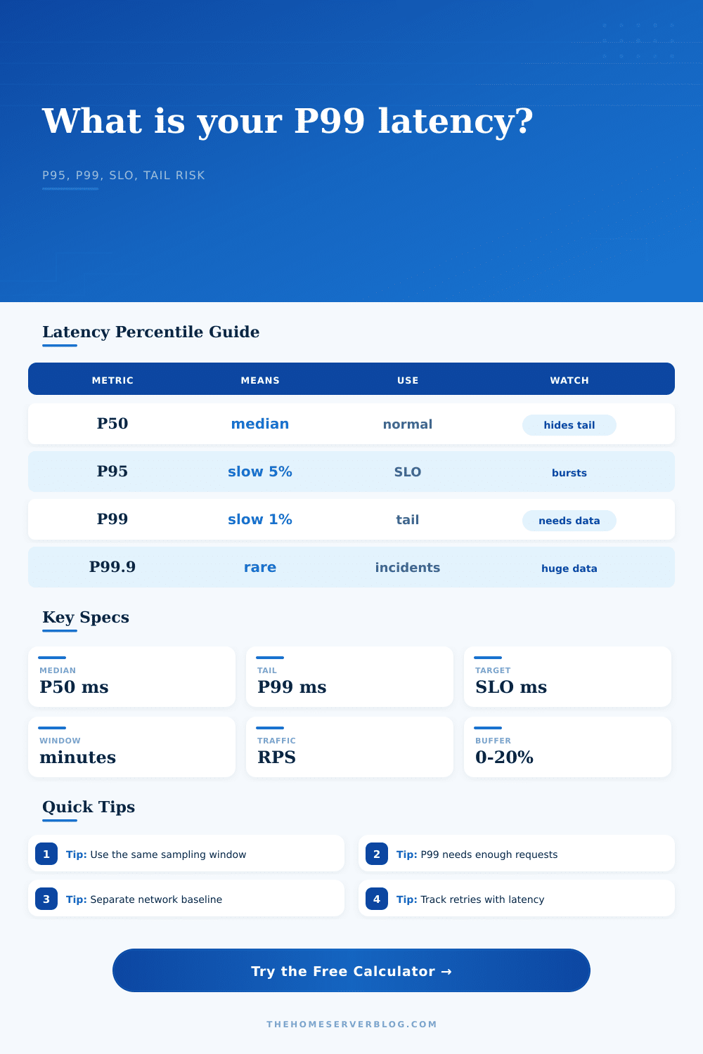
Finally, pay attention to the ratio between the P99 and the P50. That’s the P99/P50. If your system has a low ratio it means that it’s consistent. A high ratio indicates either a noisy neighbor, cold start, or some kind of queue issue. Something is intermittently blocking the pipeline, so most requests go through quickly but occasionally they does not.
The page includes a handy table of reference that shows how the percentile numbers behave for different amounts of request, reminding you that P99 needs a large sample size to become statistically significant. It takes thousands of requests to smooth out the outliers. Don’t trust the P99 if you’ve only got a hundred requests.
Don’t overlook the network baseline. Small services are easily dominated by WiFi jitter and VPN tunnel overhead. A ten-millisecond service might result in a thirty-millisecond actual tail latency, since the network adds another twenty. Spending time trying to blame the app for slow networking is wasted effort. Isolate the network layer from the application layer by measuring its round-trip time independently and plugging it into the tool. That way when troubleshooting, you separate the two layers and know exactly which one needs tuning. After all, how can you tune something if you can’t measure it?
The tool has some useful built-in presets that provide a feel for how much SLO should be for a database query, a media server, or a reverse proxy. Don’t accept those without thinking about it though. You’re different. Your network is different. Your workload is different. Your hardware is different. Let the presets tell you what goes into it, then change them to reflect your values.
You don’t want an arbitrary number. You want to understand how reliable your system is. If you see a little SLO headroom, you know you’re pushing up against the limit. A big one means you can grow some more. Slower doesn’t mean unreliable. Slower means you need to manage it.
There’s no getting around the tail. There will be some requests that is slower than others. The question is: How slow do things get before it affects my users? That’s where the calculator comes in. It lets you see that edge clearly, so you’re no longer guessing if your setup is good enough. And that change in perception is what makes something a hobby project vs. It is a robust service.
The median is nice to have; the tail is what keeps you up at night. Watch out for it.