Queue Depth Latency Calculator
Estimate how storage queue depth, IOPS demand, block size, cache policy, and device class affect home server latency before VMs, NAS shares, or databases feel stalled.
Queue Depth Latency Estimate
| Storage Target | Typical Service Latency | Comfortable Queue Depth | Home Lab Use |
|---|---|---|---|
| Single HDD | 8 to 12 ms random | 1 to 4 | Bulk NAS shares, archive data, low-concurrency backups |
| HDD mirror or small RAIDZ | 6 to 10 ms mixed | 2 to 8 | Light VM storage, media libraries, family file shares |
| SATA SSD | 0.10 to 0.35 ms mixed | 4 to 32 | Proxmox boot pools, Docker data, VM datastores |
| NVMe SSD | 0.03 to 0.12 ms mixed | 16 to 128 | Databases, build caches, high-density virtual machines |
| Replicated network storage | 1.5 to 6 ms mixed | 8 to 64 | Ceph labs, iSCSI targets, clustered virtualization tests |
| Metric | Formula Used | Why It Matters | Healthy Range |
|---|---|---|---|
| Mixed service time | Read share × read ms + write share × write ms | Combines read and write device behavior into one operation time | Lower is better |
| Effective IOPS capacity | Harmonic mixed IOPS × queue efficiency | Prevents read-heavy numbers from hiding slow synchronous writes | Above demand |
| Utilization | Adjusted demand / effective capacity | Latency rises sharply as utilization approaches saturation | Under 0.70 |
| Queue wait | Service ms × utilization / (1 - utilization) | Approximates the waiting portion of response time | Near service ms or less |
| Payload throughput | IOPS × block KiB / 1024 | Shows whether the workload is latency-bound or bandwidth-bound | Below link limit |
| Scenario | Typical Demand | Queue Depth Starting Point | What To Watch |
|---|---|---|---|
| Light SMB/NFS share | 50 to 300 IOPS | 2 to 8 | Rotational disks become jumpy during metadata scans |
| Proxmox VM datastore | 500 to 5,000 IOPS | 16 to 64 | Multiple VMs can stack small random writes quickly |
| Database with fsync | 200 to 20,000 IOPS | 8 to 32 | Sync writes reveal cache and SLOG behavior |
| Backup ingest window | Large blocks, lower IOPS | 4 to 16 | Throughput can saturate before latency looks bad |
| Photo or mail indexer | Many 4 KiB to 16 KiB ops | 16 to 64 | Small files amplify queue wait and CPU path overhead |
| Layer | Queue Behavior | Added Latency Clue | Useful Check |
|---|---|---|---|
| SATA AHCI | NCQ up to 32 commands | Deep queues rarely help HDD random reads | Compare QD1 and QD32 random latency |
| NVMe | Many queues with many entries | Parallelism helps until CPU or thermals limit service | Watch p95 latency, not only peak IOPS |
| virtio-scsi / virtio-blk | Guest queue feeds host queue | Too many VMs can create unfair queue stacking | Cap per-VM queue depth for noisy guests |
| iSCSI / NFS / SMB | Network and protocol queues add path time | Fast media can still feel slow over a busy link | Measure round trip path latency separately |
| ZFS sync writes | ZIL/SLOG path controls commit latency | Queue depth cannot hide slow durable commits | Test with sync on and realistic block sizes |
This calculator uses a planning model for queueing and device service behavior. Real results still depend on firmware, controller cache, filesystem settings, CPU load, thermal throttling, and the exact benchmark profile.
You pick out the perfect drive for your home lab. You want to make sure it has high sequential read speeds. You check its endurance rating. Ensure that it physically fits into your chassis.
Boot up your virtual machines and everything is sluggish. Your database hangs and the mouse lags. Open up your task manager and see that the disk usage are hovering around forty percent. You assume the drive is just slow, but the real culprit is usually invisible. But most of the time, the real problem is actually queue depth.
What is Queue Depth and How It Affects Speed
Storage speed is typically thought of as a highway. How fast does it go? Is it wide or narrow? Traffic goes by if it’s wide. It is a good mental model until you remember that storage devices doesn’t serve up just one request at a time. Instead they serve up a pile of requests. That pile is called the queue depth.
If there’s a big enough pile for the drive to chew through slowly, then each individual operation wait in line. Your human brain interprets that wait time as lag. Lag is latency. That’s an abstract concept. The calculator on this page turns that abstraction into concrete numbers.
You choose the shape of your workload and it shows you exactly how much waiting is occurring before the drive even begins to work. Your choice of storage target profile tells the tool what the physical speed of the drive is at serving a single request. For example, a spinning hard drive might take around eight to twelve milliseconds to locate a random block on a platter. An NVMe drive will do so in microseconds. That is the floor: the minimum amount of time it takes the drive to perform its job for that request.
That number is queue depth, which is the number of requests stacked up while that one request is getting served. Eight virtual machines asking for something at the same time and your drive can only serve one? Those other seven are waiting. That’s what the tool measures: how much wait time occurs based on how saturated the device is.
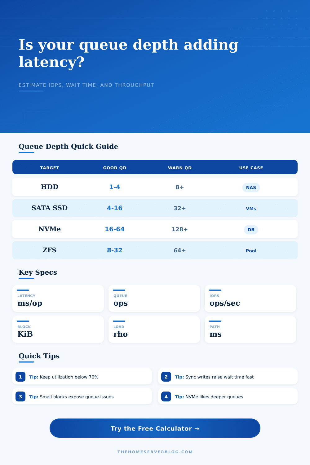
The tool also includes a reference table, which I found useful. This breaks out comfortable queue depths for each type of device. For example, a single hard drive will be happy with a queue depth of one through four. Anything over eight, and the delay starts to skyrocket. This happens because the mechanical head jump around way too much.
Solid state drives behave different. Because there’s no moving part, they’re able to handle parallel requests far better. A typical enterprise SATA SSD can comfortabley handle a queue depth of thirty-two. And NVMe drives can handles even more.
But just because they can handle more doesn’t mean you want to throw them all at the drive simultaneously. You still want to keep your use below seventy percent. That’s the sweet spot. That is where performance stay consistent. Beyond that, small demands result in huge jumps in wait time.
And then there’s the write cache policy. Is this a write-through, write-back, or sync? Writes are often slower than reads, particularly when you are forcing the data to be written to durable media right now. So for example a media server streaming out sequential video files isn’t going to see queue depth pressure as quickly as a database that’s doing synchronous writes.
And so if what your output says is that your queue has been waiting a long time, then that means you have more IOPS demand than the device can keep up with clearing out its backlog. Maybe you’ll think “oh, I’ll just buy a faster drive and it’ll go away.” Sometimes it does. More often the solution is easier. Staggering backup jobs or reducing the number of simultaneous active client will reduce the queue depth without having to spend any money.
The throughput number in the result is a good way to check that. Throughput lets you know whether it is a latency or a bandwidth problem. High throughput, low IOPS means your blocks are big; such as with a backup stream. It is easy on the queue. Small blocks (like database pages) generate lots of IOPS and soon start to clog the queue. It’s not about moving data around, it’s about forcing the storage controller to take individual trips, lots of them.
So really all the tuning of the home server comes down to consistency more so than peak performance. Some drives are faster on average, but slow down suddenly when under load. That’s worse than some other slower drives that stay consistent. And that’s where the tool come in. It will show you where those spikes is going to occur.
Capacity planning becomes a mathematical problem that you can solve, rather than a guessing game. Plug in how much load you expect, and it will tell you whether or not you have enough hardware for the crowd. If the queue wait time is high, you’ll know you need to either dial back the concurrency, or upgrade your storage tier.
What I love about this approach, though, is that it keeps you from overspending. When you keep the queue shallow, you don’t need a datacenter-grade array to run a few VMs. You only need to understand the line. Make the line short, and everything will feel smooth. That’s the secret sauce behind a responsive home lab.