HomeServerBlog path capacity planner
Throughput Bottleneck Calculator
Compare source read speed, practical link payload, CPU or encryption processing, target write speed, protocol overhead, latency behavior, and scheduling headroom to find the stage that limits a real home lab transfer.
▣Home lab throughput presets
⚙Transfer path inputs
Calculation breakdown
Stage comparison
🖥Equipment and path comparison grid
📊Derived path metrics
Minimum bottleneck throughput needed to fit the adjusted payload inside the window.
Nominal link converted to MB/s after link efficiency, profile loss, overhead, and latency.
Source read ceiling after applying parallel workers and the profile stream cap.
Estimated metadata, retries, framing, and small-file bytes added to the user payload.
📘Reference tables
Interface payload reference
| Interface | Nominal rate | Practical payload | Common home lab limiter |
|---|---|---|---|
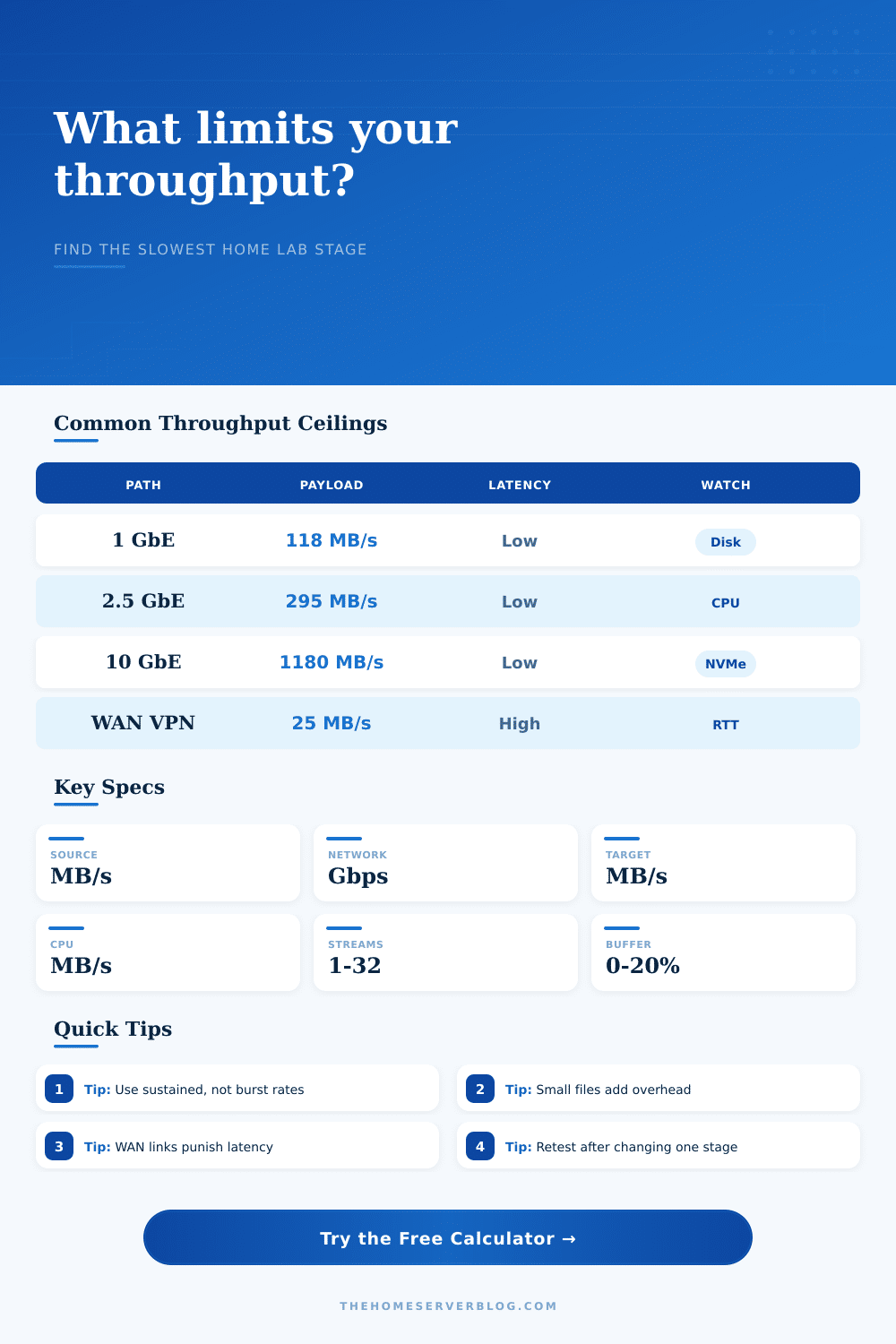
| Gigabit Ethernet | 1 Gbps | 110-118 MB/s | Single HDD, antivirus scan, SMB signing, old CPU |
| 2.5GbE Ethernet | 2.5 Gbps | 260-295 MB/s | SATA HDD array, USB bridge, low-end NAS CPU |
| 10GbE Ethernet | 10 Gbps | 900-1180 MB/s | PCIe lanes, NVMe thermals, ZFS sync writes, checksums |
| Wi-Fi 6 client | 600 Mbps-2.4 Gbps PHY | 70-160 MB/s | Signal, airtime contention, retries, client antenna count |
| USB 3.x SATA dock | 5-10 Gbps bus | 180-450 MB/s | Drive media, UASP support, bridge firmware, cable quality |
Path profile assumptions
| Profile | Efficiency model | Stream behavior | Latency sensitivity |
|---|---|---|---|
| Wired Ethernet file copy | High payload efficiency when MTU and NICs are healthy | Few streams usually enough | Low on LAN |
| Wi-Fi transfer | Lower payload efficiency due to airtime and retries | Moderate benefit from parallel jobs | Medium, especially with interference |
| VPN or WAN | Lower due to tunnel headers and MTU limits | Parallelism may hide RTT | High and packet-loss sensitive |
| Local direct attach | Very high bus efficiency for large blocks | Storage queues matter | Very low |
| iSCSI datastore | High sequential payload, sync behavior can bite | Queue depth matters more than copy streams | Medium for VM latency |
Typical source and target ceilings
| Component | Conservative ceiling | Healthy ceiling | What to test |
|---|---|---|---|
| Single 5400 rpm HDD | 80 MB/s | 140 MB/s | Sequential read after cache flush |
| Single SATA SSD | 350 MB/s | 520 MB/s | Sustained write, not only burst cache |
| Four-disk RAIDZ or parity pool | 180 MB/s | 450 MB/s | Mixed read/write and sync setting |
| Consumer NVMe SSD | 1000 MB/s | 3500 MB/s | Thermal throttling during long copy |
| Low-power NAS CPU with encryption | 80 MB/s | 450 MB/s | VPN, TLS, compression, checksum path |
Common project sizes
| Project | Payload size | Suggested input focus | Likely bottleneck |
|---|---|---|---|
| Photo library backup | 500 GB-2 TB | Small-file overhead and target write | Metadata or HDD |
| Proxmox host migration | 200 GB-4 TB | CPU ceiling, VM disk source, network | Source or link |
| Media NAS rebuild copy | 4 TB-40 TB | Target write and long-window headroom | HDD array |
| Offsite replication | 50 GB-5 TB | WAN Mbps, latency, tunnel CPU | Upload or RTT |
| iSCSI datastore move | 500 GB-10 TB | Queue depth, sync writes, 10GbE path | Target sync |
Reference values are practical planning ranges. Measure your own source, link, processing, and target stages with the same workload pattern whenever possible.
⚡Throughput planning tips
The gigabit connection… that wasn’t the end. It’s merely middle of the road. You can have gigabit speeds on your box but you’re never going to get gigabit speeds when you’re moving terabytes of data around your home lab. The difference between the two is the bottleneck. And it lurks within every little thing. It could be tiny protocol penalties of copying millions of small files, CPU overhead of encryption, target write cache, or source disk. And knowing what those numbers mean prevents you from sitting next to a progress bar at 3 AM while calculator runs the math for you.
First off, everyone believe what their links claim to be. A gigabit Ethernet sounds like 125 megabytes per second… except that’s raw throughput without taking anything into account in real world. You lose some of that right away to Ethernet framing and even more to TCP headers and SMB (or NFS) overhead. That’s not a problem if you’re copying big chunks of media around. But copy millions of tiny JPEG photos? Then all that chatter from the protocols will consume a large part of your available bandwidth. You must adjust tool to compensate for this overhead.
Finding the Slow Part of Your Connection
Metadata handling scale differently than block storage. This is another one of those little things that makes no difference until you find yourself squeezing a job into a four hour maintenance window. The other side of this is the storage. “Everybody thinks about the network and nobody thinks about the disks.” For example, a moddern NVMe drive can read gigabytes per second. But if your data writes to a spinning hard drive array with parity calculations on top, it might only manage two hundred megabytes per second. The bottleneck might not even be the network. Your destination can’t keep pace.
Find weakest link in the chain. Is it your TLS encryption? Or maybe your CPU is working too hard compressing the data via ZFS. Once you hit some kind of limit on how much data the system can process, throwing money at more network bandwidth won’t help, you’re wasting money for speed you don’t get.
Turns out it’s all about latency; particularly when your files are going across the network to some remote site or perhaps even via a VPN. Since single-stream transfer is badly affected by round trip time (each packet must wait for acknowledgement before sending the next), the trick is using multiple streams. Using more workers or streams hides more latency and creates a fuller pipeline. You’ll see exactly how much real-world throughput you can expect with different numbers of streams, before diminishing returns take hold. And there you go: a calculator to help you model this. It is a balance, as ever. Not enough streams? Idle. Too many? They overwhelm the small file index or hit CPU saturation, which creates another bottleneck of its own.
The second constraint is timing. Sure, you want to know if the data’s going to fit, but more importantly, are you going to get there before your deadline? That’s where window input comes into play. It allows you to specify when you have available time (e.g. You might use a weekend for a migration or an overnight backup window. Then the tool will figure out how much extra space you’ll need. If your estimated transfer time doesn’t fit within this window, it tells you that before you’ve even begun. It makes you face up to your own constraints. Sometimes you’ll realize that you’ll need to reduce the payload, add some buffer for retries, or admit that it’s just not going to fit in one pass.
This gets presented as a set of reference tables on the page, which provide you with real-world baselines of what to expect from various hardware configurations. For example, generally speaking a gigabit copper link will deliver about 118 megabytes per second, whereas a 2.5 gigabit configuration will get you closer to 295. This isn’t some theoretical max… It’s the rate at which you’re sustaining data over time, and something you can count on when planning. You can then compare your own setup against those norms and see what stands out. Your 10 gigabit connection should of be pushing out 400 megabytes per second. Something else must be wrong: it’s either your disk queue depth, your CPU, or the fact that your SSD has been thermally throttled.
In the end, that’s what throughput planning comes down to: Managing expectations. You’re not in control of physics of your hardware, but you are in control of how you feed it. Isolate each stage and test its limits. Then you’ve turned a guessing game into a solved equation.
That slowest link always wins. Find it early and save yourself time, frustration and bad decisions. Find out where the choke point is. Fix it. Or at least work around it.