Columnar Compression Ratio Calculator
Estimate compressed warehouse size, compression ratio, storage saved, and scan reduction from row data, encoding, codec, nulls, repeats, row groups, and target file format.
▣Data Warehouse Presets
▣Source Data Inputs
Estimate Breakdown
▣Current Model Signals
▣Codec and Format Reference
| Codec / Format | Typical Use | Compression Strength | Read CPU | Notes |
|---|---|---|---|---|
| Snappy | Interactive analytics | Moderate | Low | Fast default for many Parquet lakehouse workloads. |
| ZSTD | Large fact tables | High | Medium | Often a strong balance for cloud object storage and cold BI tables. |
| Gzip | Portable archives | High | Medium-high | Common and compatible, but usually slower than Snappy or ZSTD. |
| LZ4 | Fast pipelines | Low-moderate | Very low | Useful when CPU is tighter than storage. |
| Parquet | Warehouse tables | Encoding aware | Low-medium | Column chunks, row groups, statistics, and predicate pruning. |
| ORC | Hive-style analytics | Encoding aware | Low-medium | Stripes, indexes, bloom filters, and mature compression choices. |
▣Column Encoding Comparison Grid
| Encoding | Best Data Pattern | Weak Pattern | Typical Ratio Help | Warehouse Tip |
|---|---|---|---|---|
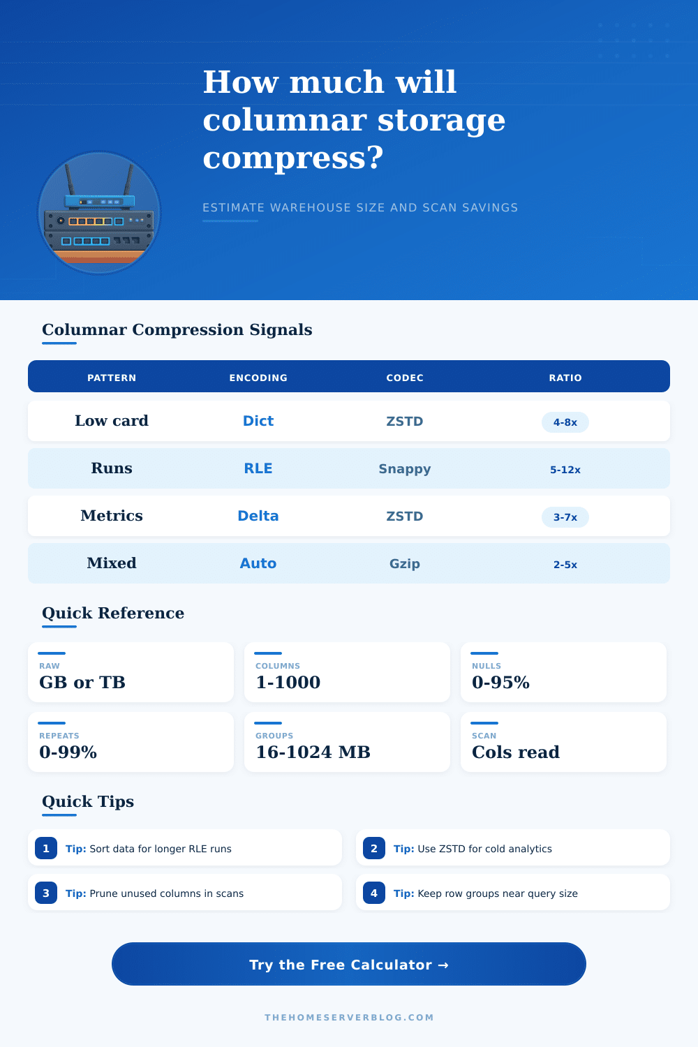
| Dictionary | Low cardinality strings, enums, categories | Unique IDs, long free text | 2x to 8x before codec | Keep category columns typed and avoid noisy variants. |
| RLE | Sorted columns with long repeated runs | Randomly shuffled data | 3x to 20x on run-heavy columns | Sort by partition, date, status, or tenant where queries allow. |
| Delta | Timestamps, counters, numeric sequences | Random high variance values | 1.5x to 6x before codec | Store times and metrics as typed numbers, not strings. |
| Bit packing | Small integer ranges and booleans | Wide decimals or binary payloads | 1.2x to 4x before codec | Use compact integer types when the engine preserves them. |
| Plain + codec | High-cardinality mixed data | Low-cardinality columns | 1.1x to 3x from codec | Acceptable fallback, but not the goal for dimensional data. |
▣Data Warehouse Preset Reference
| Preset | Pattern | Encoding | Codec | Expected Outcome |
|---|---|---|---|---|
| Parquet Fact Table | Numeric measures plus keys | Auto mixed | Snappy | Balanced size with low read latency. |
| Dictionary Dimension | Many repeated categories | Dictionary | ZSTD | High ratio and strong column pruning. |
| Clickstream Events | Wide event attributes | Auto mixed | ZSTD | Good savings if noisy JSON is limited. |
| IoT Time Series | Ordered metrics and timestamps | Delta | ZSTD | Strong compression when sorted by device and time. |
| CDC Landing Zone | Changed rows with IDs | Plain mixed | Snappy | Moderate ratio, optimized for ingest speed. |
| Customer 360 Wide | Wide profile table | Dictionary | ZSTD | Null-heavy optional attributes compress well. |
| Finance Ledger | Sorted accounts and dates | RLE | Gzip | Good ratio, but reads may spend more CPU. |
| Metrics Rollup | Aggregated numeric facts | Delta | LZ4 | Fast scans with moderate storage savings. |
| JSON Lake Export | Nested strings and payload columns | Plain mixed | Gzip | Compression helps, column pruning helps less. |
| Iceberg Analytics | Partitioned lakehouse table | Auto mixed | ZSTD | Strong size reduction with snapshot metadata overhead. |
▣Practical Tips
This calculator is a planning model. Actual compression depends on value distribution, writer version, data types, nested schema shape, partitioning, sort order, and engine-specific encoding choices.
This usually starts out well: you have a big pile of unprocessed raw JSON log data and a data warehouse that promises to take it and make something beautiful of it. So far so good; throw all your stuff into some cloud object storage. Unlimited! Cheap! It’s got to be OK right? It is usually not.
When the bill gets way too high for the month, or when query latency become unbearable, that’s when confidence melts away. And it’s usually not just because there’s a whole lot of data; it’s how that data exist on disk prior to being processed by an engine. Columnar storage changes the geometry of your data, but only if you let it.
How to Save Money on Data Storage
Input your data characteristics for each row in the table, and the calculator does the math for you. This saves you from guessing whether your mix of text and timestamps will compress, or if it will just cause higher CPU use when reading. It makes you realize that there’s no magic switch called “compression.” Rather, it’s a series of choices, beginning with how data appears on disk and ending with which codec to run across that representation.
The encoding layer gets skipped. People assume that gzip or zstd is where all the action happens. No. First the data are encoded. Dictionary encoding reduces repeating strings down to little integer pointers if you have low cardinality column such as status flags. It’s a huge reduction as it converts the text to numbers prior to being seen by compressor. An encoder can do nothing for you if your data look like random noise. Patterns makes a difference.
More than most engineer realize, sort order matters. Long strings of the same value, or adjacent values; is best for run-length encoding. User IDs in random order across files? Nothing. But if you sort by tenant ID (or some other value like a partition date) first, then write, those runs extend themselves and they’re good at compression. It is a little thing you do operationally that save you a lot on storage. The repeat percentage input and sort quality account for that. You get a feel for just how clustered your own workload really are.
Next, consider the codec choice. For interactively analyzing data, you can safely choose Snappy as your codec since it’s fast to decompress. This makes scanning cheaper by using less CPU. For big fact tables or other cold data, Zstd will give you slightly better compression at the expense of some CPU cycles. For these, storage cost trumps compute cycle. In other words: there’s no free lunch. You’re paying for either disk space or processor time.
The chart on the page makes this very clear. It suggests (as you might expect) gzip isn’t a good analytic codec, but is familiar from file archival purposes.
Another variable is nulls. Does your format handle them well? Is it compressed with high nulls? Good! Is it wasting space where you store a complete payload for a null value? Bad! If you have wide tables and lots of optional columns, then don’t query these columns when querying because it doesn’t compress very well. You should of drop the ones that aren’t used in the query. This shows up as part of the scan reduction metric which tell you how much of your database has been transferred across the wire vs. How much is sitting on disk. It shouldn’t cost you anything to move the 32 out of 40 columns you didn’t pick in your BI tool.
The point of the demo (with preset examples such as customer profiles or IoT time series) is that there are not one-size-fits-all solution to different types of data. For example, a clickstream log full of chaotic event attributes differ from a table of financial records sorted first by account number and then by date. The former benefits from delta encoding on counters, while the latter rely on dictionary compression for categorical strings. The latter leverages counter-based delta encoding. Warehouses cost money when they treat everything as if it belong in a single mold.
The last part is validation. The models are good for planning, but you’ll be surprised in the real world by distributions. Don’t test on synthetics; test with a representative sample. Apply those settings, then see what happens in the real world; how big the files turn out, how fast queries perform. There’s no magic to compression. It simply shows how well your data structure match the tools that know best how to shrink it. Match your access patterns with codec, encoding, and sort order, and storage stops behaving as if it were a bottomless pit. It begins acting like an engineered system.