Database index capacity planning
B-tree Index Size Calculator
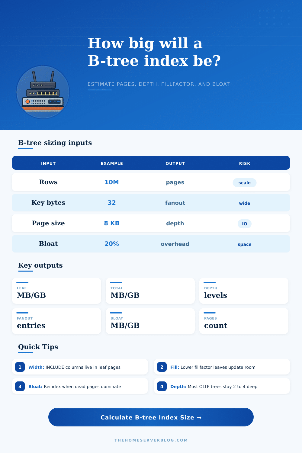
Estimate unique B-tree index leaf size, total pages, branch levels, tree depth, fanout, INCLUDE column impact, fillfactor reserve, null fraction effects, and bloat overhead.
Page math summary
Capacity indicators
| Layer | Entry math | Fanout or pages | Size | Notes |
|---|---|---|---|---|
| Leaf | Key + pointer + overhead | 0 | 0 MB | Calculated after inputs load |
PostgreSQL default
8 KB pages, heap TID references, B-tree page metadata, and optional INCLUDE columns stored at the leaf level.
InnoDB secondary
16 KB pages are common. Secondary indexes include the clustered primary key, so wide primary keys increase every secondary index.
SQL Server rowstore
8 KB pages, nonclustered row locators, fill factor settings, and included columns can heavily influence leaf size.
Oracle B-tree
Block size, PCTFREE, rowid bytes, key compression, and branch block fanout all affect leaf blocks and depth.
| Term | Calculator approximation | Typical source | What to tune |
|---|---|---|---|
| Leaf entry bytes | compressed key + INCLUDE + tuple pointer + overhead | Index tuple format | Key width, include bytes, overhead |
| Usable leaf bytes | (page size - page overhead) x fillfactor | Page layout and fill policy | Page size, fillfactor, overhead |
| Leaf pages | ceil(row count / leaf fanout) | Bottom B-tree level | Row count and entry width |
| Branch pages | ceil(child pages / branch fanout) per level | Internal pages and root | Branch levels, key width, pointer width |
| Bloat overhead | base index size x bloat percentage | Dead tuples, splits, fragmentation | Reindex, vacuum, rebuild policy |
| Index type | Best for | Size behavior | Lookup pattern | Watch out for |
|---|---|---|---|---|
| Unique B-tree | Primary keys, unique constraints, equality, ranges | Predictable, often compact unless keys are wide | Point and ordered range scans | Random insert splits and bloat |
| Nonunique B-tree | Common filters and joins | May need duplicate handling or posting lists | Point, range, ORDER BY support | Low selectivity can still be large |
| Covering B-tree | Index-only reads and hot APIs | Larger leaf pages because INCLUDE data is stored there | Fewer heap lookups | Wide includes reduce fanout |
| Hash index | Equality lookups only | Often smaller for simple equality keys | No ordering or range scans | Less flexible than B-tree |
| BRIN index | Huge append-ordered tables | Very small summary pages | Block range pruning | Poor for random data distribution |
| GIN index | Arrays, JSONB, full-text terms | Can be much larger than table columns imply | Containment and token matching | Pending lists and update cost |
| GiST index | Geospatial, ranges, custom operators | Depends on operator class and splits | Nearest neighbor and overlap | Variable selectivity and page splits |
| Bitmap index | Warehouse columns with low cardinality | Compact for repeated values | Bitmap combinations | Usually poor for high-churn OLTP |
Sometimes you see that query hanging in space; sometimes you don’t, though. Sometimes the culprit isn’t the algorithm but rather the index. That’s because a bloated and sprawling index force the database engine to read pages that do not contain any useful data. You don’t start thinking about indexes as things with trees and byte counts until inserts slow down or the index begin gobbling up your storage budget.
Math, baby: time to count the nodes. So how much? The overhead is calculated automatically by the calculator above. You enter the width of each key in your rows and number of rows, and it does the math for you. But to understand where this overhead comes from, we need to take a look at B-trees‘ internal design.
Why Indexes Take Up Space
Each index entry has an associated cost. This includes length of the key data, a pointer to the corresponding real row in the table, and some metadata used to maintain the tree’s shape. For instance, PostgreSQL adds up to a dozen bytes of overhead with an alignment pad and a tuple header on each and every entry. That doesn’t sound like much per-row, until you multiply it times ten million rows, and you’ve got megabytes of wasted storage.
The largest lever available is your key width. An eight byte integer key uses half the space of a sixteen byte UUID. And a wider primary key will propagate into all of your secondary indexes, since each has to stores the clustered key reference too. That’s the width you’re paying for in everything. To account for it, the tool lets you specify your key payload (including column sizes). It then shows you how much more space each leaf node will take if you expand your key with covering columns to avoid a heap lookup. It’s a tradeoff between space efficiency and read speed.
The other issue is fillfactor. If you set it to 90 percent, then every page will have ten percent free space on it. That’s so that if you need to update that table later, you’ll leave some space free rather than forcing page splits. Because page splits are an expensive operation (they rewrite data, which can mess with the index), you want to avoid them as much as possible.
If you have a lot of random inserts and/or updates to columns in your index, maintaining a low fillfactor will slows down performance. However, it will keep things running smoothly once things get going. It just means more room has to be allocated initially. The calculator accounts for this cushion so you can see what your base size will be before it starts getting all wonky from being broken up.
Bloat is a silent index-killer. It slowly kills the efficiency of an index. Updates and deletes result in the creation of dead tuples that vacuum cleans up…eventually. To give you a sense for how much more (or less) your production environment will be bloated relative to a fresh build, we have an input to specify the bloat percentage.
Let’s say that after accounting for the base size of your indexes you calculate your database consumes fifty megabytes. If bloat accounts for twenty percent then you’re now looking at sixty megabytes on disk. Those extra twenty megabytes won’t speed any queries. They simply slow down scans by taking up buffer pool space.
How many levels? Well designed OLTP indexes has typically two to four levels. In other words, a point lookup can be accomplished with just a handful of random I/Os. As your data blows up (or your keys get too wide) then the tree becomes deeper. Every added level increases seek time for each operation.
The tool uses the fanout to calculate branch levels automatically. This shows how likely it is that your index design will stay lean at scale. These calculations are based off reality with reference tables for various db engines. By default, PostgreSQL and SQL Server use an eight kilobyte page, whereas InnoDB uses a sixteen kilobyte page. That alters the fanout considerably.
A wider page can hold more entries, which decreases the tree’s depth and improves seek performance for larger data sets. But the wider the page, the fewer number of pages you’ll get within a given buffer pool size. There is a tradeoff between depth and cache efficiency.
Columns This is a very effective optimization, but it has an important caveat. If all your non-key data lives on the leaf pages, then you can serve queries directly off the index, without costly lookups into tables. But the tradeoff is that each extra column shrinks the number of rows you fit onto a page. And if you get fewer rows per page, then you have more pages to go through, and a taller tree to traverse. So consider the time saved by reads vs You should of also consider the added storage and maintenance costs.
Size is also impacted in subtle ways by null handling. How much space does a null value take up within the key structure? It depends upon the database. You have an option to specify a fraction of nulls and this will decrease the average payload if many of your keys are often empty. It’s a niche optimisation but one that adds precision to the estimate.
At the end of the day, this is why sizing an index is a matter of expectation setting. There’s no way to get limitless speed, zero storage, and no-maintenance forever. Pick two. The calculator gives you a visual representation of the tradeoff ahead of time, before it becomes a production issue. Knowing the relationship between bloat, fillfactor, and key width will help you build great-performing indexes that don’t take up your whole disk array. It makes it an engineering decision instead of a guessing game.