HomeServerBlog WAN sizing tool
SD-WAN Link Aggregation Calculator
Estimate usable aggregate throughput, best single-flow Mbps, failover capacity, and SLA score from three WAN links, latency, loss, traffic split, tunnel overhead, QoS reserve, flows, and bonding mode.
After tunnel overhead, QoS reserve, loss, and mode efficiency.
Mode-specific estimate for one large TCP or UDP flow.
Remaining usable capacity after the largest active link drops.
Latency, loss, failover, split balance, and headroom score.
Calculation breakdown
Highest effective single-link capacity after loss and reserves.
Difference between fastest and slowest active links.
Normalized traffic distribution used for weighted health math.
Planning action from SLA score and failover capacity.
Per-flow load balancing
New flows spread across links, but a single large transfer normally stays on one path.
Weighted ECMP
Flow placement follows link weights, useful when broadband circuits differ in speed.
Packet striping bond
Packets from one flow can cross multiple links, so latency skew and loss matter more.
Tunnel bonding with FEC
Overlay bonding can repair loss and use multiple links, but extra parity and headers reduce wire rate.
Application-aware steering
Voice, video, POS, and SaaS traffic can prefer the path that best matches SLA rules.
Active-backup failover
One link carries service while standby capacity waits for an outage or brownout event.
| SLA class | Latency target | Loss target | Failover target |
|---|---|---|---|
| Voice and real-time control | Below 80 ms weighted latency | Below 0.5% weighted loss | 1 to 3 seconds for conversational apps |
| Video and VDI | Below 120 ms weighted latency | Below 1.0% weighted loss | 3 to 8 seconds before sessions feel rough |
| Business apps | Below 180 ms weighted latency | Below 2.0% weighted loss | 10 seconds or less for most SaaS workflows |
| Bulk transfer and backup | Below 300 ms weighted latency | Below 4.0% weighted loss | 30 seconds may be acceptable for queued work |
| Bonding mode | Aggregate model | Single-flow model | Planning note |
|---|---|---|---|
| Per-flow load balancing | Sum of effective links times flow diversity | Fastest healthy single link | Best with many independent sessions such as browsing, SaaS, and branch users. |
| Weighted ECMP | Sum of effective links with split mismatch penalty | Fastest healthy single link | Good when traffic shares roughly match actual circuit capacity ratios. |
| Packet striping bond | Sum of links with strong skew and loss penalty | Can use several links for one flow | Works best when links have similar latency and low loss. |
| Tunnel bonding with FEC | Sum of links after parity and tunnel efficiency | Multi-link with repair overhead | Useful when loss repair matters more than absolute top speed. |
| Application-aware path steering | Policy-adjusted sum of SLA-qualified paths | Usually fastest link per app class | Prioritizes application experience rather than maximum Mbps. |
| Active-backup failover | Primary active link only | Primary active link only | Simple and predictable, but backup bandwidth is idle until failover. |
| Link mix | Strength | Weak point | Best SD-WAN behavior |
|---|---|---|---|
| Fiber plus cable | High bandwidth and low latency | Shared local conduit or ISP path may still fail together | Weighted ECMP or per-flow load balancing. |
| Fiber plus LTE or 5G | Different physical failure path | Higher latency, carrier NAT, and variable loss | Active backup or app-aware steering for critical traffic. |
| Starlink plus fixed wireline | Useful rural diversity | Latency swing and obstruction-driven loss bursts | Application-aware steering with conservative bonding. |
| MPLS plus broadband | Predictable private path and cheap extra capacity | Policy complexity and asymmetric bandwidth | App-aware steering for voice and ERP, broadband for bulk. |
| Result signal | Healthy range | Watch range | What to adjust |
|---|---|---|---|
| Usable aggregate | Above busy-hour demand plus reserve | Less than 25% headroom | Reduce tunnel overhead, adjust split, or add link capacity. |
| Best single-flow Mbps | Enough for the largest transfer or stream | Far below aggregate capacity | Use bonding only if apps need one-flow acceleration. |
| Failover capacity | Can carry critical traffic after one link loss | Below QoS-reserved critical traffic | Reserve more QoS or choose active backup with a better standby path. |
| SLA score | 80 or higher | 60 to 79 | Reduce latency skew, loss, failover time, or split overload. |
If you’ve ever been frustrated with your internet connection because it takes too long to download big files even though your internet service provider advertises blazing-fast speeds, you’re familiar with this issue. Raw bandwidth isn’t the same as usable throughput. When you take a speed test, you may think that’s the amount of capacity you have to use. The truth include more variables.
How does traffic flow through several different links? What impact do latency skew, packet loss and tunnel overhead has on advertised speed? Effective network planning starts with understanding the gap between what you pay for and what you get.
Why Your Internet Speed Is Slower Than You Think
The vast majority of folks will think that doubling the number of connection is just going to double their throughput. The calculator shows how intuitive fallacy leads them astray here. It factors in tunnel overhead, which subtracts some fraction of your bandwidth from whatever you’re using to protect and encapsulate traffic. Fail to consider this and you risk making capacity plans that are more hopeful then intended. “Sure I can do video chat!” But now those encrypted headers is hogging half your bandwidth.
It also factors in QoS reserves, so that bulk downloads don’t crowd out control or voice traffic. That’s especially valuable when a big update starts syncing.
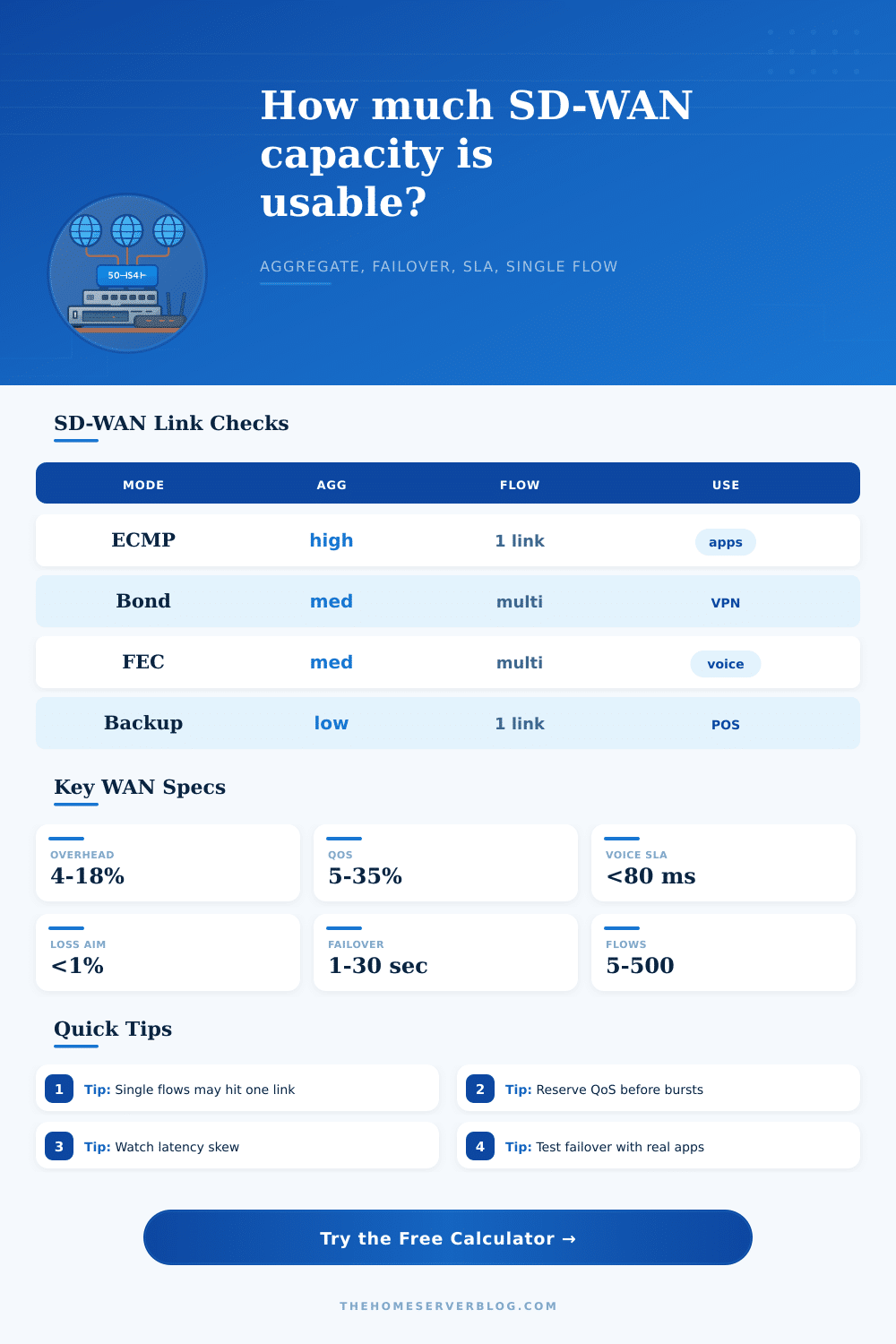
Bonding modes also matter a lot in terms of their single-flow performance. While per-flow load balancing is good for general office browsing by spreading various users/applications over your links, it doesn’t accelerates a single large download. Packet striping can split a single flow, but it requires similar latency on your links. Otherwise, some packets will arrives before others and get reordered, reducing TCP throughput. As the reference table shows, each mode trades raw speed against some combination of stability/reliability. Rather than simply seeking out the biggest number, you should of select a mode based off what your actual applications require.
Another negative impact on performance comes from latency skew. Take, for example, combining a fast fiber link with a slower cellular back-up; you’ve now combined connections running at vastly different speeds. Your jitter, the delay between these two paths. Gets in the way of virtual desktop session (they’ll be laggy) and disrupts VoIP calls.
These penalties factor into the calculator’s SLA score, which is important because this number indicates if the connection is good enough to meet your needs. Having a large aggregate speed number doesn’t help if the underlying quality isn’t there. Sure, you may have lots of capacity, but if packets starts dropping intermittently, or arriving out of order, the application won’t know what to do with them.
But you shouldn’t ignore failover capacity until it’s needed. Active-backup configurations maintains an unused backup circuit in case of failure. That’s reliable because retail point-of-sale terminals are mission-critical. However, this configuration wastes money on unused bandwidth. A bonded setup uses all links simultaneously for maximum efficiency, but the complexity of failover logic become harder with one path degrading.
Is staying connected during an outage your top priority? Or do you want maximum throughput? It depends. This isn’t a free solution; it is just a set of tradeoffs that align with your budget and level of risk tolerance.
SD-WAN planning is about managing expectations, not going for top speed. Speed tests can be misleading because they don’t show your actual usable throughput. Managing it means considering flow behavior, loss, and latency. By matching your real application needs to your hardware capabilities, you make the network less mysterious and more predictable. The frustrating bottleneck becomes a reliable utility.