MTBF to Reliability Calculator
Convert MTBF into exponential mission survival, fleet no-failure probability, expected failures, and a confidence range for home lab hardware planning.
| Mission Scenario | Typical MTBF | Mission Time | Single Survival |
|---|---|---|---|
| Enterprise SSD media in a NAS cache | 2,000,000 hr | 1 year | 99.56% |
| Rack switch electronics in a home lab | 500,000 hr | 1 year | 98.26% |
| Surveillance hard drive service year | 1,000,000 hr | 1 year | 99.13% |
| 72-hour hardware burn-in run | 250,000 hr | 72 hr | 99.97% |
| Mission as MTBF Fraction | Formula | Survival Probability | Failure Probability |
|---|---|---|---|
| 0.01 x MTBF | e^(-0.01) | 99.00% | 1.00% |
| 0.10 x MTBF | e^(-0.10) | 90.48% | 9.52% |
| 0.50 x MTBF | e^(-0.50) | 60.65% | 39.35% |
| 1.00 x MTBF | e^(-1.00) | 36.79% | 63.21% |
| Single-Unit Survival | 5 Units All Survive | 20 Units All Survive | 100 Units All Survive |
|---|---|---|---|
| 99.9% | 99.50% | 98.02% | 90.48% |
| 99.0% | 95.10% | 81.79% | 36.60% |
| 98.0% | 90.39% | 66.76% | 13.26% |
| 95.0% | 77.38% | 35.85% | 0.59% |
| Output | What It Means | Use It For | Common Mistake |
|---|---|---|---|
| Single survival | Chance one device lasts the mission | One server, one disk, one switch | Treating it as guaranteed life |
| Fleet survival | Chance no unit fails in the fleet | Drive pools, AP fleets, camera sets | Ignoring fleet size |
| Expected failures | Average count over total exposure | Spares and maintenance planning | Rounding small means to zero |
| Confidence range | Approximate Poisson count range | Risk communication | Calling it an exact guarantee |
When you plan your hardware for a project, you must consider the likelihood that the hardware will survive the length of your project. Many people look at the Mean Time Between Failures (MTBF) rating for the hardware to determine its likely lifespan. However, the MTBF isnt the likelihood that your specific hardware will survive your specific project; it is the average failure rate for the population of that type of hardware.
To determine the likelihood that your hardware will survive the length of your project, you must use a mathematical model. One of the simplest models for calculating the likelihood of survival is the exponential model. The exponential model states that the failures of hardware components happen at random intervals.
How to Estimate If Hardware Will Survive a Project
The exponential model is useful for calculating the likelihood of survival for electronics in particular after the initial period of “early” failures of those electronics. The exponential model does not account for the “wear-out” failures of electronics, but it is still useful for determining the likelihood of survival based on the total amount of time that the electronics will be powered on. The total amount of time that the electronics will be powered on (in hours) is more important than the total length of time that the electronics will be in use (in hours) because the powered on time is a more accurate indicator of the stress that will be placed upon the electronics.
In order to calculate the likelihood of survival for the electronics for your project, you must first determine the length of the mission of the electronics. You must convert the length of the mission into the number of hours that the electronics will be in use. You must multiply the number of hours that the electronics will be in use by the duty cycle and the environment factor for the electronics.
The duty cycle for the electronics is important because it indicates the number of hours per day that the electronics will be in use. The environment factor is important because it indicates the amount of stress that the electronics will experience while in use in there specific location. Another variable in the equation is the size of the fleet of those electronic hardware components.
Many people tend to overlook the size of the fleet of electronic hardware components. If an individual unit of hardware has a high likelihood of surviving its mission, the likelihood that all of the units in a large fleet will survive their missions is lower. The calculator accounts for the size of the fleet; it determines the likelihood that zero electronic hardware units in the fleet will fail during the length of the missions.
The size of the fleet is, thus, another factor that individuals who plan electronic hardware for projects must consider. Another figure that the calculator provides is the number of expected failures of the hardware components. You can calculate the number of expected failures by dividing the total amount of time that the hardware will be in use by the MTBF of that hardware.
This number is an estimate of the average number of failures that the hardware will sustain during its missions. This number is not a guarantee that the hardware will fail the number of times represented by the expected failures figure. The number of failures can be estimated with a Poisson approximation to provide a confidence range for the expected failures.
This confidence range indicates the percentage of confidence that the actual number of failures will fall within a range of two numbers. This figure can be used to determine how many spare units of hardware should be purchased for the project. Another feature of the calculator is the target reliability input.
Rather than entering the length of the project to determine the likelihood that the hardware will survive the length of the project, the target reliability input allows for the entry of the percentage of reliability that you desire for the hardware. The calculator can then calculate the length of the project that will allow for the hardware to have that percentage of reliability. This feature can be used to set cycles for the hardware to replace failed hardware components.
Additionally, if a percentage of reliability for a type of hardware component can be determined, that percentage can be used to evaluate if the hardware component can be used in a project of a certain length. Many people make mistakes with the use of the MTBF ratings for hardware components. One of the mistakes that people make is to assume that the MTBF for a hardware component is the minimum length of time that the hardware will last.
This is not true of the MTBF; some hardware components will fail before the MTBF, and some will fail after the MTBF. Additionally, the exponential model makes assumptions about the time period that is being measured for the hardware components; it only accounts for the powered on time of the components. Time spent repairing and recovering the hardware components isnt accounted for in the model.
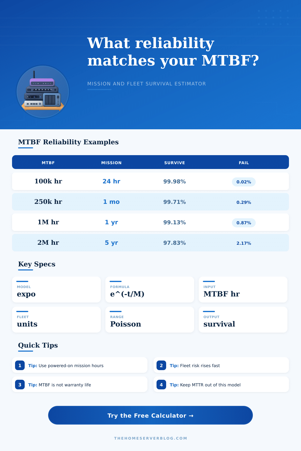
The calculator provides a number of reference examples that show how the survival rate of the hardware components changes when the length of the mission changes in relation to the MTBF of those hardware components. The examples show that if the length of the mission is shorter than the MTBF of the hardware components, then both the single-unit and the fleet survival probabilities will be high. However, as the length of the mission increases, the survival probability for both individual units and fleets of hardware components will decrease.
Additionally, the relationship between mission length, fleet size, and survival probability of the electronic hardware components is not linear; small changes in mission length or size of the fleet can have a large impact on the survival probability. By running the same set of inputs through the calculator, but altering the duty cycle or the environment factor for the hardware components, it is possible to determine the importance of each variable for the hardware component. If altering the environment factor significantly reduces the survival probability of the hardware component, then the environment factor for that hardware component is a critical variable.
If altering the environment factor has little impact upon the survival probability of the component, then the environment factor is not the most important variable for that hardware component. In addition to determining the importance of each variable for a specific hardware component, it is also possible to use the model to compare the survival probabilities of different hardware components. For example, it is possible that a hardware component with a high MTBF will have a low survival probability for its units if the length of the missions that the units will perform is very long.
Additionally, it is possible that if each mission for the hardware component is of short length, that a hardware component with a lower MTBF may still be acceptable for the projects. Thus, the calculator allows individuals to compare the survival probabilities of different brands, models, and types of hardware components. The two most important figures that the calculator can determine are the figure for the survival of the fleet of hardware components and the number of failures in the expected failure range.
Each of these figures can help to determine both the average and the worst case scenarios for the hardware. By considering both figures, an individual can make certain that there is a plan in place for both the average and the worst case scenarios. The model provides an estimate for how the hardware will survive based off its MTBF; this estimate can help to an individual to make decisions regarding reliability of hardware components.