HomeServerBlog database throughput planner
Provisioned Throughput Cost Calculator
Plan provisioned read and write capacity units from item size, read consistency, peak burst multiplier, target utilization, autoscale buffer, and the throughput already assigned to the table.
Selected workload profile
DynamoDB Small Table models a compact application table with moderate reads, a small write stream, mixed consistency, and enough target headroom for normal bursts.
Capacity breakdown
Utilization and headroom
DynamoDB provisioned capacity
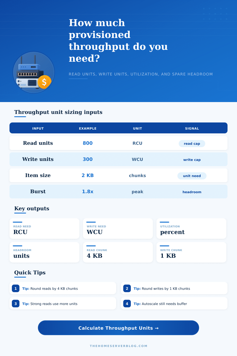
Reads and writes are separate lanes. Read size rounds by 4 KB chunks, write size by 1 KB chunks, and strong consistency changes read capacity demand.
Cosmos DB RU/s containers
Request units combine reads, writes, queries, and indexing work into one pool, so item size and query shape matter more than lane separation.
Cassandra capacity units
Throughput is usually bounded by partition distribution, compaction, consistency level, and node resources rather than a single table unit counter.
MongoDB document throughput
Working-set fit, index coverage, write concern, and shard key balance determine how far provisioned hardware can carry document reads and writes.
Redis or KeyDB memory service
Operations are usually CPU, network, and memory-bound. Headroom should be watched with latency, evictions, and hot-key concentration.
SQL primary with read replicas
Provisioning is instance or pool based. Read and write pressure interact through locks, log flush, buffer churn, and replica apply lag.
| Unit rule | Calculator logic | Capacity meaning | Planner note |
|---|---|---|---|
| Read item chunk | ceil(item KB / 4) | Each 4 KB read chunk consumes capacity per read operation. | Items just over 4 KB double read chunk count. |
| Write item chunk | ceil(item KB / 1) | Each 1 KB write chunk consumes capacity per write operation. | Small payload growth can raise write units quickly. |
| Strong read factor | strong share x 1.0 plus eventual share x 0.5 | Mixed consistency has a weighted average read capacity cost. | Use the percentage of reads that truly require latest data. |
| Target floor | demand / target utilization | Converts peak demand into provisioned units with operating margin. | Lower targets create more headroom before throttling. |
| Workload pattern | Typical read mix | Typical write mix | Capacity warning |
|---|---|---|---|
| Product Catalog Reads | High read rate, mostly eventual reads | Low writes except imports and price changes | Cache miss storms can make the read lane hot first. |
| Session Store | Moderate reads with freshness needs | Write-heavy updates and TTL churn | Short-lived rows can stress write capacity and partitions. |
| IoT Telemetry Writes | Low read rate during ingestion | High append-heavy writes | Item size and partition key spread dominate write headroom. |
| Leaderboard Updates | Read bursts around rankings | Frequent counter or score writes | Hot keys may throttle even when table average looks safe. |
| Utilization band | Modeled max | What it means | Operating response |
|---|---|---|---|
| Comfortable | Under 55% | Provisioned capacity has room for routine variance. | Keep alarms, then reduce only after a full traffic cycle. |
| Target zone | 55% to target | Capacity aligns with target utilization and buffer planning. | Good steady-state range for provisioned tables. |
| Tight | Target to 100% | Current units can serve modeled demand but have little spare room. | Raise units, reduce strong reads, or prewarm before peaks. |
| Short | Over 100% | Modeled demand exceeds one or both provisioned lanes. | Increase capacity or smooth the burst before relying on autoscale. |
| Preset | Provisioned shape | Main pressure | Best first check |
|---|---|---|---|
| DynamoDB Small Table | Small read and write lanes | Mixed consistency reads | Confirm average item size and strong read share. |
| Hot Partition API | Larger total units with skew risk | One tenant or key family | Check partition key cardinality and hot keys. |
| Multi-Tenant SaaS | Balanced read/write capacity | Noisy tenants and bursts | Review per-tenant routing, quotas, and alarms. |
| Launch Day Surge | High buffered capacity | Autoscale lag and retries | Pre-provision the peak instead of waiting for alarms. |
Building a database table used to be a bit of a guessing game; you guess some numbers that seem reasonable and roll out app. Then you sit around waiting for the inevitable first traffic spike to let you know whether you guessed right. Unfortunately, most times, you didn’t.
Engineers naturaly begin by estimating a steady state. After all, they’re comfortable with averages. But averages deceive in context of capacity planning. The danger isn’t on a quiet Tuesday afternoon. It’s when your cron jobs all wake up at the same time, when a marketing campaign launches, or when you’re doing an important Friday evening deploy.
How to Plan Your Database Capacity
The above calculator does the math for you, and knowing what goes into it will help you not trust results without checking them yourself. First of all: check out item size. The system’s rounding rules round up, so even though a 1.6 kilobyte average row might seem small, it actualy makes a difference. In write scenarios, writes uses one-kilobyte chunks, so that rounding rule makes it true that an eight-byte item is going to cost you just as much throughput than a three-byte item. Likewise, crossing the four-kilobyte boundary on reads doubles your cost immediately. People get that wrong by looking at byte counts and thinking linearly, capacity pricing is in steps.
A second level of complication is in the consistency settings: strongly consistent reads will show you the most up-to-date version, but use double the read capacity of eventually consistent reads. In other words, if you use strong consistency for only 35% of your traffic, you have changed your base usage by a meaningful amount. The tool does math for you based off this mix. All you have to do is tell it where your queries really can’t afford stale data. For many applications, you can use eventual consistency for everyday browsing and keep strong reads for the critical path stuff. These include session validation and payment confirmation.
Theory meets reality when discussing burst modeling (traffic doesn’t come smoothly); instead it comes as waves because of retry storms from failing downstream services, user behavior patterns, or cache evictions. Without a burst multiplier on your steady-state throughput, you’re provisioning for a world that doesn’t exist; so applying a burst multiplier to your steady-state throughput provide a realistic peak demand number. This means the resulting capacity numbers takes into account headroom for unexpected load spikes and jitter.
So what happens if you’re running at 100% capacity? That’s where your safety valve (target utilization) comes in. There is no wiggle room or room for error, so it is dangerous to run a table at full capacity. For example, instead of aiming for 100%, aim for 70%. This leaves a thirty percent free buffer. And that buffer soaks up all the noise, so you don’t throttle. Cost obsessed? Tighten it up. Hungry for stability? Loosen it up. The reference tables on page lay out the effect of different uses on operational risk, and those comfortable numbers allow you to sleep while those tight ones makes you stay up monitoring dashboards.
So what about Autoscale? That would seem to be the answer. However, it has latency. If your alarm triggers an autoscaling capacity increase, there is a delay before those new units become available. And while we wait on those to come online, where does all that excess traffic go? It goes into the autoscale buffer input which is additional provisioned capacity over and above your calculated requirement in order to account for that ramp time. In other words, it’s insurance in case there’s a gap between detection and response. You should of pay for it monthly to prevent any downtime while waiting for scaling up.
These inputs are interesting when compared to other database architectures that pool all requests as a unit, where a single request is a mix of both reads and writes. Nothing wrong with that, unless one side spikes. In that case you don’t know whether it’s because of reads or writes. By separating them, DynamoDB forces you to size each lane separately. For example, let’s say your product catalog gets hammered by readers, but writes stays flat. You only have to adjust read capacity, since you don’t need to over provision the write lane just because the read lane is busy.
A session store is not like an IoT data receiver and the tool’s presets mirror typical real world scenarios. Write-heavy append-only streams vs. Short-lived data is read-heavy. Understanding which scenario your workload falls into allows you to check if the outputs make sense. Does it say I need some huge amount of write capacity for a static catalog? Something is off here: either you’ve mixed up reads/writes, or typed item size wrongly.
The last metric is spare throughput. This metric indicates safety, since a positive number means you have some headroom while a negative number means you are already oversold. If you plan ahead, you can use those signals to determine whether or not you need to right-size prior to your next traffic event, which is always better than having to react after the fact.