Storage IOPS to Throughput Calculator
Convert random or mixed storage IOPS into practical throughput, then compare it against disk class, queue depth, and network link limits for a home server or lab NAS.
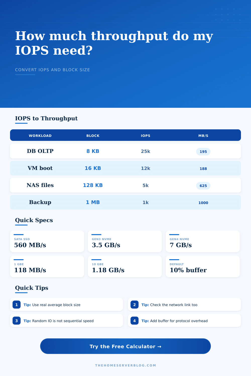
Formula used: throughput in MB/s = IOPS × block size in KB ÷ 1024, then adjusted for selected overhead.
Full Breakdown
| IOPS | 4 KB | 8 KB | 16 KB | 64 KB |
|---|---|---|---|---|
| 1,000 IOPS | 3.9 MB/s | 7.8 MB/s | 15.6 MB/s | 62.5 MB/s |
| 10,000 IOPS | 39.1 MB/s | 78.1 MB/s | 156 MB/s | 625 MB/s |
| 50,000 IOPS | 195 MB/s | 391 MB/s | 781 MB/s | 3125 MB/s |
| 100,000 IOPS | 391 MB/s | 781 MB/s | 1563 MB/s | 6250 MB/s |
| Link or Bus | Practical MB/s | Approx GB/s | Useful Storage Ceiling |
|---|---|---|---|
| 1 GbE | 118 MB/s | 0.12 GB/s | Single HDD or light SSD NAS |
| 2.5 GbE | 295 MB/s | 0.29 GB/s | Fast HDD mirror or entry SATA SSD |
| 10 GbE | 1180 MB/s | 1.18 GB/s | SATA SSD pool or NVMe-backed NAS |
| PCIe 4.0 x4 NVMe | 7000 MB/s | 7.0 GB/s | Local scratch and direct attach NVMe |
| Workload Pattern | Typical Block Size | Read Mix | Planning Note |
|---|---|---|---|
| Database OLTP | 8 KB to 16 KB | 60% to 80% | IOPS matters more than sequential rating |
| VM datastore | 16 KB to 64 KB | 55% to 75% | Boot storms raise queue depth quickly |
| Media library | 128 KB to 1 MB | 80% to 95% | Throughput and network limit dominate |
| Backup repository | 512 KB to 1 MB | 20% to 50% | Write path and link ceiling are critical |
| Home Lab Project | Input Example | Throughput Result | Secondary Check |
|---|---|---|---|
| Small Proxmox cluster | 20k IOPS at 16 KB | 313 MB/s raw | Fits 2.5 GbE with little headroom |
| PostgreSQL WAL device | 18k IOPS at 8 KB | 141 MB/s raw | Latency is usually the harder target |
| 10GbE NAS backup | 1.2k IOPS at 1024 KB | 1200 MB/s raw | Consumes nearly a full 10GbE link |
| Nextcloud thumbnail cache | 35k IOPS at 8 KB | 273 MB/s raw | SATA SSD IOPS can matter more than link |
NVMe drives? Seven gigabytes per second! You can’t get any faster then that!” you think as you sit down to improve your home server.
Then when you go to run a database on it, the system start stuttering. You check the metrics. Why isn’t it going so fast? Oh yeah: the disk’s barely moving any data. (The box says it have high IOPS.)
Understanding Throughput and IOPS
That’s the trap of storage systems. You went out and bought yourself a fast drive to move data around. But something about the timing killed the performance. Why was there confusion? Because you mixed up two different things: throughput and IOPS. They’re related, yes. But they’re not the same thing.
Consider it as a library. The librarian pulls out books from the shelf every second. How fast are they pulling them? This is IOPS. How big are these books? This is throughput.
So if the librarian has a book with one hundred bytes of data and they pull one thousand of them off the shelf every second, that’s low throughput even though the IOPS are high. They have to move all that little data. If instead they have heavy encyclopedias and pull one thousand of those off the shelf every second, now the throughput increase because there is more data coming through.
The calculator will do the math for you. It takes the raw number of operations and turns it into megabytes per second based off the block size you entered.
That’s where people make their planning mistake. People assume high IOPS automatically means high throughput. But small blocks keep the total amount of data flowing very slowly. Even at the highest speeds the drive can run, the data doesn’t get any faster. Block size is the real variable here.
Eight kilobyte block are common for database transactions. Sixteen kilobytes are typical for virtual machine boot storms. Bigger chunks are common for streaming media or large file backups. Some can go as big as a whole megabyte. You’ll plug in those numbers, and the tool will adjust its output accordingly.
Twenty-five thousand IOPS at eight kilobytes looks very different than twenty-five thousand IOPS at sixty-four kilobytes. One requires fast drives with low latency. The other requires a big network pipe. Plug in the wrong number and you could of end up buying more storage speed than you need (or less network capacity). It’s a tiny detail, but one that makes a difference in your budget.
Then there’s the network ceiling to consider. You might think “I have fast storage” but your NAS connect over a one gigabit ethernet port. It is capable of about one hundred and eighteen megabytes per second. The rest gets eaten up by protocol overhead. This is why it’s important to check the link limit.
That’s where this tool come into play. It helps visualize your headroom. Is your demand on the storage more than the cable can handle? Build a large RAID array and many will find their bottleneck is the network switch. The thing people get wrong. Rarely is the storage the limiting factor in a home lab, usually it’s the connection.
Latency and queue depth come into play as well. You don’t really notice them unless the system starts crawling. If you have high IOPS and shallow queue depth then the drive is taking care of requests immediately. If you have high IOPS and deep queue depth then the drive is overwhelmed and you’ll wait longer for the request.
The calculator estimates this latency so you can see if your drive class matches the workload. Is the workload aligned with your drive class? Backup throughput is probably doable on a spinning hard drive. Random IOPS used by a virtual machine datastore won’t be. You want the right tool for the job, not the fastest one.
Once you get that, you begin to shop differently. No longer are you searching for the biggest number on paper. Instead you’re seeking the right combination. That SATA SSD could work great for your Nextcloud server. It might look good on paper compared to an NVMe drive, but its strength is a good match for the random access pattern. It’s about having enough speed without wasting money.
So that’s when you get the hardware. And then you see the difference. There is no more stuttering. The backups complete on schedule. The database answer in a flash. Turns out, you didn’t even need the seven gigabyte drive after all.
You finally understood what those numbers mean. The library analogy is valid. It is not about how many books you own but how fast can you find the one book you want to read, and read it without delay?