Noise Figure Calculator
Model RF receiver chains with Friis cascade math, front-end cable loss, source temperature, filter bandwidth, and the SNR target for your home lab radio link.
Full cascade breakdown
| RF element | Typical gain/loss | Typical noise figure | Practical note |
|---|---|---|---|
| Short SMA pigtail | -0.2 to -0.8 dB | Same as loss | Small but visible before an LNA |
| 10 m RG-58 at UHF | -2 to -4 dB | Same as loss | Often dominates weak-signal chains |
| SAW or cavity filter | -1 to -5 dB | Same as loss | Best after a low-noise gain stage when possible |
| GaAs pHEMT LNA | 15 to 25 dB | 0.4 to 1.5 dB | Strong first-stage choice for SDR receivers |
| Passive mixer | -5 to -8 dB | 6 to 10 dB | Needs enough preceding gain for low system NF |
| Formula | Expression | Units | Use in calculator |
|---|---|---|---|
| Noise factor | F = 10^(NF/10) | Ratio | Converts each stage from dB to linear |
| Friis cascade | Ftotal = F1 + (F2-1)/G1 + ... | Ratio | Combines cable, LNA, and IF stages |
| Noise temperature | Te = 290 x (F - 1) | K | Shows receiver noise as an input temperature |
| Thermal density | N = -174 + 10 log10(B) | dBm | Baseline input noise across bandwidth |
| Detectable signal | MDS = floor + SNR target | dBm | Estimates signal level needed at the input |
| Receiver scenario | Bandwidth | SNR target | Noise figure target |
|---|---|---|---|
| LoRa or telemetry gateway | 125 to 500 kHz | 6 to 10 dB | Under 3 dB preferred |
| General SDR voice/data | 12.5 kHz to 2 MHz | 10 to 12 dB | Under 5 dB acceptable |
| Wi-Fi OFDM receiver | 20 to 80 MHz | 18 to 25 dB | 4 to 7 dB typical |
| GPS/GNSS front end | 1 to 4 MHz | Correlation dependent | Under 2 dB after antenna LNA |
| Microwave downconverter | 1 to 50 MHz | 12 to 18 dB | LNA placement is critical |
| Project setup | Equipment count | Primary concern | Healthy result |
|---|---|---|---|
| Rooftop SDR antenna | Coax, bias tee, SDR | Loss before gain | LNA at antenna, NF below 3 dB |
| LoRaWAN gateway | Filter, LNA, concentrator | Adjacent-channel filtering | Low-loss filter after LNA |
| Wi-Fi lab receiver | Antenna, FEM, radio | Wide bandwidth floor | Enough SNR after 20 MHz noise |
| Satellite L-band chain | Dish feed, LNA, cable, SDR | Outdoor cable attenuation | High LNA gain before cable run |
After weeks of fussing with dish alignment and the antenna tuning, you’re now hearing the static growing louder. But you can’t make it go away. The problem is never that you can’t hear. Something invisible in your system, between your antenna and radio, are drowning out the universe.
That’s what a radio’s “noise figure” measures: How much the universe gets drowned by your own equipment. It is not just some number printed on a data sheet; it is the number that tells you how badly your receiver are interfering with itself.
Understanding Radio Noise Figure
The math runs in this calculator above. You plug into it the gain of your amplifier, loss of your cable, and then noise contribution of your mixer. Then Friis formula kicks in and tell you what’s what. It spits out one number which represents total degradation of signal to noise ratio. This one number mean the difference between hearing a whisper or just a shout.
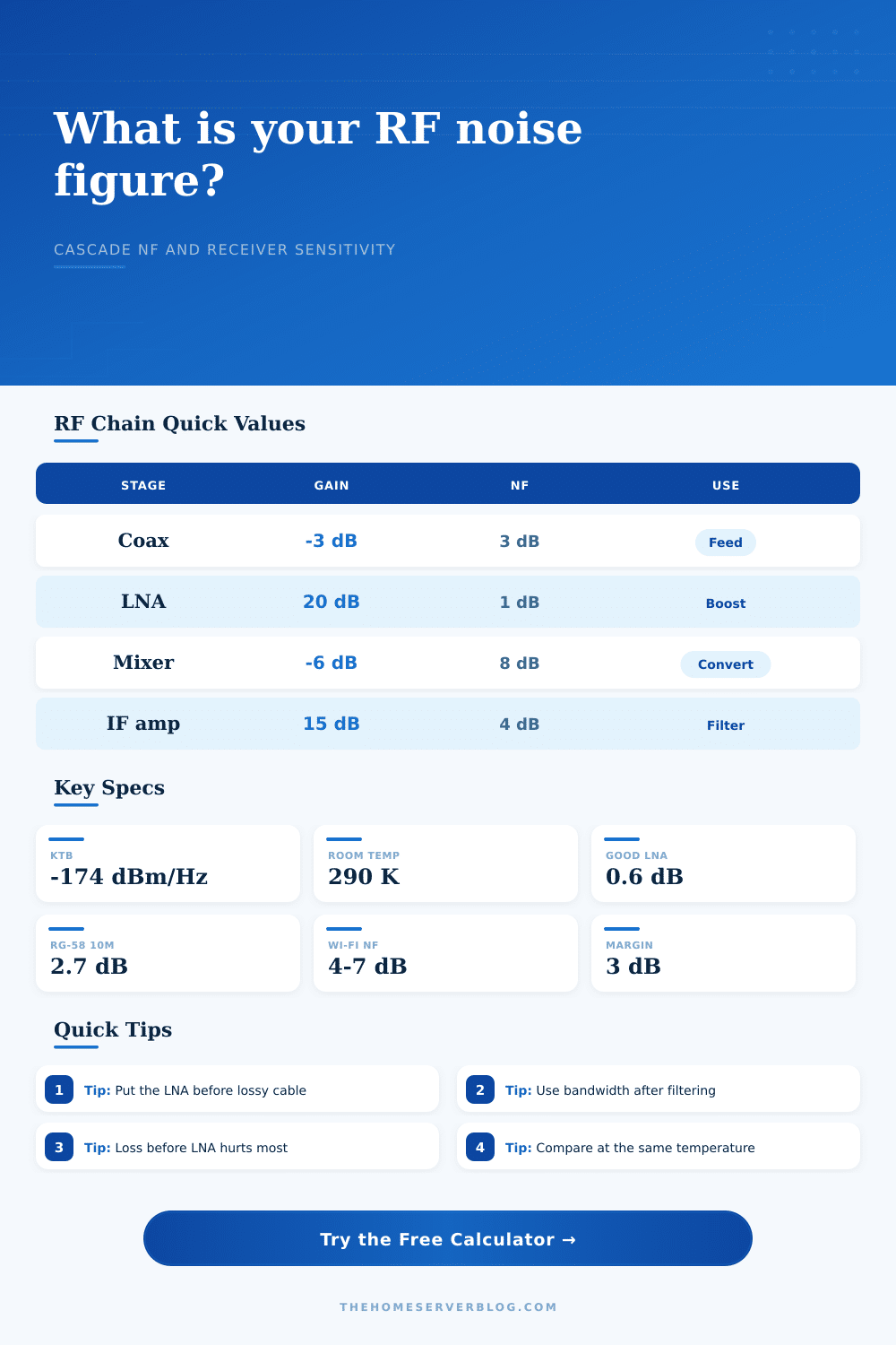
What that number means is far more important than simply making it as small as possible. That is the first golden rule of RF design: the first stage in any receiver chain will determine what follows. Placing a low noise amplifier right after antenna reduces the noise contribution of all components downstream. Putting a long length of coax between the antenna and the amplifier just amplifies whatever noise the coax generate. The coax becomes the attenuator, raising the noise floor before signal is even amplified. A two decibel loss before the amplifier add two decibels to your system noise figure. That’s a direct tax on sensitivity. Usually it’s cheaper and more effective to move the gain nearer the source than to buy better radio.
The other tricky factor is bandwidth. Receiver comparisons often involve comparing apples to oranges because many builders don’t consider how many frequencies they’re actualy monitoring. For example, a wideband software defined radio that scans twenty megahertz of spectrum will have far more noise then a narrow band radio tuned into a single twelve point five kilohertz channel. By allowing the user to define effective noise bandwidth, the calculator normalizes for this.
How can you reduce the noise level? One way is to filter out all unwanted spectrum before analog to digital converter. That lowers the noise floor. It doesn’t affect the signal, just makes it easier to hear over background. This is where many design go awry. Mixer stages are notorious for being noisy and introducing a lot of loss too. Conversion losses may be six to eight decibels in passive mixers. It show up as additional noise figure in the cascade. Depending on how much gain you had at the front end, it could drive system noise figure through the roof. You can see typical numbers for each from the reference tables on page. A GaAs pHEMT amplifier may bring 15 decibels gain with under a decibel of noise. Your mixer may then suck down five decibels of signal and give you back seven decibels of noise. Do the math and you’ll know what’s the bottleneck.
Another factor that affects things is temperature, but not as much as folks believe. By default, calculators assumes a source temperature of two hundred ninety Kelvin, or room temperature for those like me who don’t speak heat science very well. The lower your source temperature (like with an antenna hanging outside in cool night air), the better (slightly). You can tweak this input into the calculator. For most home labs, you won’t be far from standard conditions and sticking with defaults is fine. Tweaking this one should of been more important if you’re operating in extreme environments.
It’s a balance between linearity, gain and noise. Sometimes we’re not going for the lowest noise figure. Strong nearby signals can produce intermodulation distortion if there is too much gain. Don’t use so much gain that you overload the mixer, but use just enough to mask the noise of following stages. With the tool, you can see what changes will affect your minimum detectable signal. You can change a filter or add in an attenuator.
In the end, creating a good receiver is all about compromise. Infinite gain and no noise just doesn’t happens. It’s up to you as the builder to determine where loss occurs and where amplification are added. The numbers point the way; your ear confirms it. You know the chain is working when the static dissapears and the faint signal appears. That’s the payoff of doing the math correctly.