Frequency Reuse Calculator
Estimate RF channel reuse distance, channels per sector, site capacity, and co-channel margin for Wi-Fi, cellular, private LTE/5G, LoRa, and fixed wireless plans.
Frequency Reuse Results
| Cluster N | Reuse Factor | D/R Ratio | Typical Use |
|---|---|---|---|
| 1 | 1.000 | 1.73 | Single-frequency networks, dense Wi-Fi with low power |
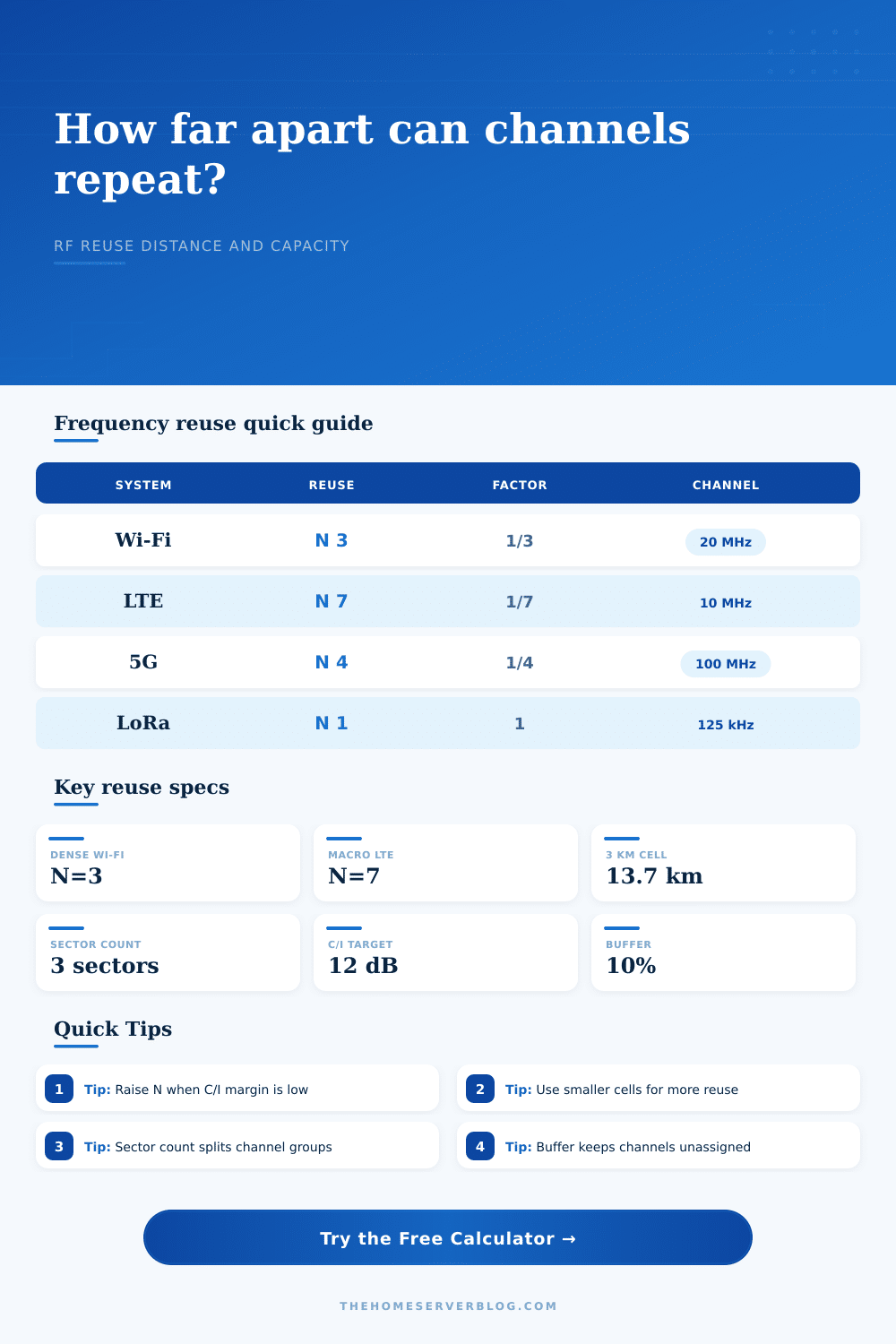
| 3 | 0.333 | 3.00 | 2.4 GHz Wi-Fi channel 1/6/11 layouts |
| 4 | 0.250 | 3.46 | Moderate private LTE, 5G, or outdoor AP reuse |
| 7 | 0.143 | 4.58 | Classic cellular planning with stronger isolation |
| 12 | 0.083 | 6.00 | Conservative sites with high co-channel protection |
| Radio System | Common Channel Width | Usable Planning Count | Reuse Note |
|---|---|---|---|
| 2.4 GHz Wi-Fi | 20 MHz | 3 non-overlap | Reuse distance matters because only 1/6/11 are usually practical. |
| 5 GHz Wi-Fi | 20, 40, 80 MHz | Varies by DFS | Wider channels reduce available reuse groups quickly. |
| 6 GHz Wi-Fi | 20 to 160 MHz | Many 20 MHz blocks | More spectrum helps, but power class and AFC rules may apply. |
| LTE FDD/TDD | 5 to 20 MHz | License dependent | Sectorization and PCI planning are separate from frequency reuse. |
| 5G NR mid-band | 40 to 100 MHz | License dependent | Massive MIMO can support tighter effective reuse than N suggests. |
| LoRaWAN | 125 kHz | Region dependent | Spreading factors also influence capacity and interference. |
| Planning Condition | Typical C/I Target | Path Loss Exponent | Practical Signal Check |
|---|---|---|---|
| Open outdoor RF path | 9 to 12 dB | 2.0 to 2.7 | Use larger N when there are clear line-of-sight paths. |
| Suburban cellular grid | 12 to 18 dB | 3.0 to 3.8 | Terrain clutter and antenna downtilt improve isolation. |
| Indoor enterprise Wi-Fi | 15 to 25 dB | 3.5 to 5.0 | Walls help reuse, but hallway bleed can dominate. |
| Directional fixed wireless | 18 to 30 dB | 2.0 to 3.5 | Antenna pattern and side-lobe control matter more than distance alone. |
| Project | Starting N | Typical Radius | Primary Constraint |
|---|---|---|---|
| Home 2.4 GHz AP layout | 3 | 20 to 40 m | Only three clean 20 MHz channels |
| Warehouse Wi-Fi | 3 or 4 | 25 to 60 m | High shelves create aisles and reflections |
| Private CBRS campus | 4 or 7 | 0.2 to 1.0 km | SAS grant, EIRP, and building penetration |
| LTE macro overlay | 7 | 1 to 5 km | Neighbor list and sector interference |
| LoRaWAN rural gateways | 1 to 3 | 2 to 10 km | Duty cycle and spreading factor airtime |
| Fixed wireless ring | 4 or 9 | 1 to 8 km | Antenna azimuth and channel width |
If you’ve ever worked in an office full of people yelling over one another, you’ve experienced the fundamental issue with radio frequency planning. Noise cancels out your message. That’s what engineers refers to as interference. There are only so many channels, and when too many voice try to speak on any given channel, they drown each other out.
The solution? Divide up available bandwidth into channels. Reuse those channels without getting in each others’ way. Use a calculator like this one to do the math for you. Enter your desired isolation and cell radius. There you go! No more manual calculation of hexagonal cluster geometry required.
How to Plan Your Radio Channels
Every time you design a new site plan, you turn geometric shapes into something practical: how many channels. The reuse factor, often denoted as N That brings us to what I call the heart of it all. The reuse factor, or N. N represent how many times a pattern appears in space. Think of N as the number of cell that repeat the same set of frequencies.
So the bigger N is, the farther apart those cells can be and the less likely co-channel interference will come near the end user. That’s good because it preserves the quality of the signal. However, the more cells there are, the fewer channels per site, which results in lower potential capacity. Finding the sweet spot is never an intuitive process, which is why you should crunch the numbers.
How close do you want the signal-to-interference ratio? It should be enough so that your modulation scheme can decode data reliably. Keep in mind that the inputs becomes part of the actual environment you are deploying in. In particular, the choice of channel bandwidth matters. If you deploy a Wi-Fi network on the 5 GHz band using 80 MHz channels you have much fewer unique frequency blocks to play with.
Using 20 MHz gives you more distinct frequency blocks to play with, but there’s a tradeoff between bandwidth and available channels. Accordingly, the tool adjust the channel count. It illustrates how rapidly your usable spectrum runs out as you open up the spigot on your pipes. More bandwidth isn’t only faster, it eats into the reusable set.
The table of references on the page spells this out nicely. It illustrates the tradeoffs for various radio systems and how they map to typical reuse factors. In a similar way, sectorization also carves the pie up into slices that point in different directions. Instead of using one antenna that broadcasts in all directions, you’re using three antennas pointing in different directions (each 120 degrees). You can be much more aggressive about reusing those frequencies in the neighboring cells.
Why? Because the physical directionality of the antennas points them away from the interferers. That’s why the calculator divides the total pool of channels by the number of sectors you have. It will give you an accurate picture of how many actual carriers each sector can accommodate. Don’t fall victim to the trap of thinking every antenna at a site has access to entire spectrum license.
A hexagon is an idealized model that doesn’t describe reality. In practice, there are walls, hills, trees, and other types of vegetation, which distort and reflect the signal, creating interference. You can tweak these environments with the path loss exponent parameter. An open field has lower signal loss, so signals go farther and interference happens sooner. That means you need more isolation. A concrete building block the signal quickly, so you can tighten up the reuse.
Enter the path loss exponent, which the tool uses to calculate the co-channel margin, the margin of safety between your desired distance and potential interference from neighboring repeaters. If it comes out in the red, game over: your design won’t work in the real world. Respect the planning buffer. It’s tempting to go all-out and max out every kilohertz of spectrum you can get away with. But that’s a recipe for instability.
If radar is detected, Dynamic Frequency Selection systems will drop channels. Neighbors could deploy additional routers. Hardware fails. Reserving a ten percent buffer for guard bands and the unexpected helps ensure a strong network. The calculator subtracts this buffer from your theoretical capacity. What it shows you is what you’ll realisticaly be able to deliver. Better to have a bit less on paper than to have a network that drops under stress.
It is more than a physical problem; it is also a management problem regarding frequency reuse. Think of the calculator as a sort of scenario tester. How wide does the channel have to be? What happens if you make the antenna higher? What if you make it lower? You will begin to see these sorts of ripples throughout your design. Use it. But don’t use it as an end answer.
Begin conservatively with your cluster size. Then work your way down until you break through the interference. It isn’t just about covering it; it’s about doing so with a clean signal strong enough to carry your data load. When you get the spacing correct, all that remains is your signal. And what you’ve got is what you need.