RTT to Bandwidth Calculator
Estimate practical TCP throughput from round-trip time, receive window, MSS, packet loss, link speed, parallel streams, and protocol overhead.
Full Calculation Breakdown
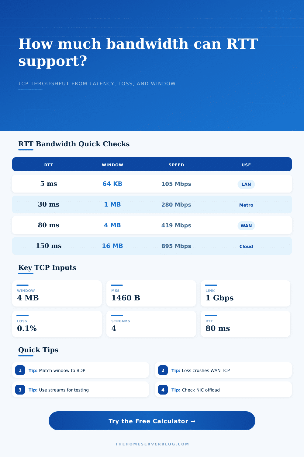
| RTT Scenario | 1 MB Window | 4 MB Window | 16 MB Window | Home Lab Read |
|---|---|---|---|---|
| 2 ms same rack or switch | 4.19 Gbps | 16.78 Gbps | 67.11 Gbps | Window is rarely the limiter |
| 10 ms local ISP or metro | 839 Mbps | 3.36 Gbps | 13.42 Gbps | 1 GbE fills easily |
| 40 ms regional cloud | 210 Mbps | 839 Mbps | 3.36 Gbps | Window scaling starts to matter |
| 90 ms cross-country WAN | 93 Mbps | 373 Mbps | 1.49 Gbps | Streams or larger buffers help |
| 180 ms satellite or distant VPN | 47 Mbps | 186 Mbps | 746 Mbps | Loss and buffer sizing dominate |
| Connection Type | Typical RTT | Common Link Rate | Suggested MSS | Planning Overhead |
|---|---|---|---|---|
| Same-switch Ethernet | 0.2-2 ms | 1-10 Gbps | 1460 bytes | 5-10% |
| Home Wi-Fi client | 4-25 ms | 150-900 Mbps | 1360-1460 bytes | 15-25% |
| Fiber internet | 5-35 ms | 300-2000 Mbps | 1460 bytes | 10-15% |
| WireGuard site VPN | 25-120 ms | 50-1000 Mbps | 1320-1420 bytes | 15-20% |
| Satellite internet | 45-650 ms | 25-250 Mbps | 1360-1460 bytes | 20-25% |
| Packet Loss | TCP Effect | What to Check | Home Lab Symptom |
|---|---|---|---|
| 0-0.01% | Usually clean | Window and link cap | Stable iPerf runs |
| 0.05% | Noticeable on WAN | Bufferbloat and retries | Fast start, uneven finish |
| 0.1% | Major single-flow limit | Wireless quality and drops | Backups underperform |
| 0.5%+ | TCP collapses quickly | Cabling, signal, queue loss | VPN and sync jobs crawl |
| Reference Item | Value | Why It Matters | Calculator Field |
|---|---|---|---|
| Ethernet MTU | 1500 bytes common | Leaves 1460 byte TCP MSS over IPv4 | MSS |
| Jumbo MTU | 9000 bytes typical | Raises MSS but requires end-to-end support | MSS |
| BDP | Bandwidth x RTT | Minimum data in flight to fill the path | RTT and link |
| TCP window scaling | RFC 7323 | Allows receive windows above 65,535 bytes | Window |
| VPN encapsulation | MTU drop likely | Smaller MSS avoids fragmentation | MSS and overhead |
You’re on a gigabit fiber line. Speed tests say you have it. For three hours, you wait as your backup job crawl along at a quarter of that rate. You double-check your NIC speed. Check the switch ports. Everything appear right.
Typically, the culprit is hidden: it’s the relationship between the time it takes for your data to reach its destination vs. How fast it does so. Delay isn’t just delay; it’s a constraint on capacity that plays off your TCP window size to calculate effective throughput. When your window isn’t large enough for round trip, the pipe is half-empty all the time. Half the time your bandwidth sits idling while you wait for an acknowledgment.
Why Your Internet Is Slow Even With Fast Speed
When you plug in your loss rates and recieve window, and then factor in your round-trip time, the calculator above does the math for you (and spares you from guessing at conversions and coefficients). It combines loss-limited TCP performance with window-limited throughput into something that shows you what you can actualy sustain.
For most folks, bandwidth is thought of like a static ceiling. Not so. Bandwidth is a product off buffer size and latency. That product are known as the bandwidth-delay product. It’s the number of bytes that need to be in flight to get link fully used. You’ll never fill the pipe if your TCP receive window isn’t equal to or larger than this product. Doesn’t matter how good your cable is or how fast your disk is. The protocol is throttling you by waiting for space to clear up before it sends more data.
High-latency links has a silent killer: loss. A tiny amount of packet loss will trigger retransmissions that crush your throughput on long paths. In a LAN environment with a round trip time of only 2 ms, you lose a packet and it costs you microseconds. The connection bounces right back. But on an eighty millisecond latency WAN link across the country, that loss event cause a stall in data flow for seconds before recovery. This happens either due to a timeout or a retransmission window. That effect compounds very rapidly. This is why distant VPN tunnels or satellite internet feels sluggish even though the raw speed might be decent. The protocol spends more time recovering from errors than actualy moving new data.
The page also has some reference tables showing what window size maps to what latency scenario. As you’ll note, with a ten-millisecond link and a one-megabyte window, you’re capped at about nine hundred megabits per second. This is fine for home use. But with a one-hundred-millisecond latency, the same window limits your effective speed to less than one hundred megabits.
Opening multiple parallel streams tend to be the solution. These are possible using tools like iPerf these days or just by using moddern file protocols. Open multiple streams. Each has its own window. Between all of them, they fill up the pipe. This is a smart workaround to a basic limitation in the protocol.
How long does it actualy take? Measure your round-trip time while running a backup job or whatever else takes up bandwidth and consumes the link. An idle-time ping will tell you precisely nothing about how it perform when you want it to perform at peak. When the link is busy, queueing delays build up as bufferbloat falsely increases your latency. For simplicity’s sake, the calculator use a static RTT. Real networks are dynamic. Use the worst-case consistent latency you see under load (not the best-case idle ping) for planning purposes. That provides a realistic ceiling.
And then there’s protocol overhead. This takes away from your payload. It includes TCP headers, IP headers, and Ethernet frames. If you use a VPN, it also include encryption headers. This shrinks the effective maximum segment size. You also deal with airtime overhead and contention if you’re on Wi-Fi. The calculator lets you make a margin for this. A five-percent overhead is good on a nice clean copper line. Twenty-five might be closer on a noisy wireless client. The margins keeps you from getting numbers that are just raw wire speed (it makes sure you have usable data).
These are the variables of your system, and they’re what you tune. A big file being moved on a high latency link? Bump up the TCP window scaling. Testing one stream? Brace yourself for limits. Open some more streams. Got some packet loss? Fix the signal strength or fix the cabling. When the input matches the real world, so do the numbers.
You’re not fighting the hardware. You’re working with the protocol. That’s why understanding that dynamic turns an annoying bottleneck into a solvable equation. Your pipe could of only been as full as you make it.