HomeServerBlog TCP performance planner
TCP Window Scaling Calculator
Estimate bandwidth-delay product, receive window size, RFC 7323 window scale shift, per-flow throughput, and parallel flow count for LAN, WAN, VPN, NAS, and lab replication links.
Full TCP window breakdown
1G Ethernet NIC
125 MB/sSmall windows are usually enough on low-latency LANs; RTT under 1 ms often keeps the BDP below 128 KB.
2.5G Multi-Gig
312 MB/sNAS backups over a home switch may need a few hundred KB of receive window when RTT stays near 1 ms.
10G SFP+ Lab
1.25 GB/sHigh local throughput depends on storage, CPU offload, driver buffers, and window scaling above classic TCP.
VPN Gateway
RTT boundEncrypted WAN paths usually need bigger windows and several flows because tunnel overhead reduces efficiency.
Wi-Fi 6 Backhaul
70-85%Airtime contention and rate shifts lower practical efficiency, so use measured throughput instead of PHY rate.
NAS Storage Stack
IO boundSMB, NFS, ZFS, disks, and cache can cap throughput even when the TCP receive window is large enough.
Cloud VM Edge
WAN RTTPublic internet transfers often require megabytes of in-flight data to approach line rate across regions.
Container Cluster
many flowsService meshes and overlay networks add headers, but many simultaneous flows can hide a small per-flow window.
| Scale shift | Multiplier | Max receive window | Where it fits |
|---|---|---|---|
| 0 | x1 | 64 KB | Legacy TCP, short LAN RTT, low-speed links, and compatibility testing. |
| 2 | x4 | 256 KB | 1G LAN with slightly higher RTT or small VPN links. |
| 4 | x16 | 1 MB | 2.5G LAN transfers, SMB backup jobs, and modest WAN paths. |
| 6 | x64 | 4 MB | 1G WAN around 30 ms RTT or 10G LAN with a few milliseconds RTT. |
| 8 | x256 | 16 MB | Fast fiber, metro replication, and higher-latency 2.5G or 10G paths. |
| 10 | x1024 | 64 MB | 10G over WAN RTT, remote backup, and high-bandwidth cloud sync. |
| 12 | x4096 | 256 MB | Long-fat networks, large file movement, and lab tests across regions. |
| 14 | x16384 | 1 GB | Maximum RFC 7323 shift, reserved for very high BDP paths. |
| Path example | Link speed | RTT | BDP receive window |
|---|---|---|---|
| Short wired home LAN | 1 Gbps | 0.5 ms | 62.5 KB before margin; classic TCP often works. |
| Multi-gig NAS to workstation | 2.5 Gbps | 1 ms | 312.5 KB before margin; window scale is usually needed. |
| 10G lab storage VLAN | 10 Gbps | 1 ms | 1.25 MB before margin; storage tuning may matter as much as TCP. |
| Fiber WAN to nearby VPS | 1 Gbps | 20 ms | 2.5 MB before margin; scale shift near 6 is a common minimum. |
| Cross-country backup | 1 Gbps | 70 ms | 8.75 MB before margin; parallel flows can help test bottlenecks. |
| Remote 10G replication | 10 Gbps | 40 ms | 50 MB before margin; big windows and NIC offload are important. |
| Frame or tunnel type | Typical MTU | Typical TCP MSS | Practical note |
|---|---|---|---|
| Standard Ethernet IPv4 | 1500 bytes | 1460 bytes | Good default for most home switches, routers, and internet paths. |
| PPPoE internet | 1492 bytes | 1452 bytes | Small MSS reduction avoids fragmentation on DSL and some fiber gateways. |
| WireGuard over IPv4 | 1420 bytes | 1380 bytes | Common tunnel value; actual MSS depends on outer path and firewall clamping. |
| IPsec tunnel | 1400 bytes | 1360 bytes | Encryption headers reduce payload; verify with path MTU testing. |
| VXLAN overlay | 1450 bytes | 1410 bytes | Used in clusters and virtual networks; underlay jumbo frames can restore payload. |
| Jumbo lab Ethernet | 9000 bytes | 8960 bytes | Reduces packet rate for storage networks when every hop supports jumbo MTU. |
| Project | Typical inputs | Primary window result | Secondary tuning result |
|---|---|---|---|
| Home NAS backup | 2.5G, 1 ms RTT, 94% efficiency | About 345 KB with 10% buffer | Shift 3 is enough when base window is 65535 bytes. |
| Proxmox storage VLAN | 10G, 1 ms RTT, jumbo MSS | About 1.38 MB with 10% buffer | Shift 5 gives room while packet rate stays manageable. |
| WireGuard remote backup | 250M, 55 ms RTT, 82% efficiency | About 1.76 MB with 10% buffer | Shift 5 or 6 and multiple flows are realistic. |
| Gigabit fiber to VPS | 1G, 25 ms RTT, 90% efficiency | About 3.09 MB with 10% buffer | Shift 6 plus tuned receive buffers should approach target. |
| Remote 10G replication | 10G, 40 ms RTT, 92% efficiency | About 55 MB with 10% buffer | Shift 10 and storage validation are usually required. |
| High RTT satellite lab | 100M, 600 ms RTT, 70% efficiency | About 8.25 MB with 10% buffer | Shift 8 and parallel transfers help with queue variation. |
Formula used: required receive window in bytes equals target bits per second multiplied by RTT seconds, divided by 8, then multiplied by the selected safety buffer. Per-flow throughput is configured window bytes multiplied by 8 and divided by RTT seconds.
The NAS is plugged into your ten gigabit switch and you’ve got your primary workstation hooked up as well. You think it’s go time for fast file transfer, but progress bar just inches along. More often than not, it’s not because of the port speed or even the cable. No, it’s probably the TCP window size.
How much data can be sent without recieveing an acknowledgement back from receiver? That’s because standard TCP is tuned for low-bandwidth links. Without scaling, its windows is hard-limited to a certain size. Pair even moderate latency with high bandwidth and pipe fills immediately. The sender’s sitting idle while the link sits empty, waiting for acknowledgements that hasn’t been received yet.
How to Fix Slow File Transfers
Once you measure round-trip time and plug in your link speed, the math gets done for you by calculator above (so you don’t need to guess about unit conversions or buffer coefficients).
Imagine that the network path is like a highway. Lanes represent bandwidth. Distance from the on-ramp to the off-ramp represents latency. Most of those lane are wasted if only one car can be on the road at once, before you’re forced to wait for permission to send another. That’s called the bandwidth-delay product. It’s how many bytes must be in transit so pipe stays full.
Window scaling: Most systems these days support it, so they multiply that base window size. What’s tricky about choosing the proper shift value? If you choose a shift that’s too big, then you risk overflowing the receive buffers on older devices and embedded system in the path. Choose a shift that’s too little, and you’re leaving some performance on the table.
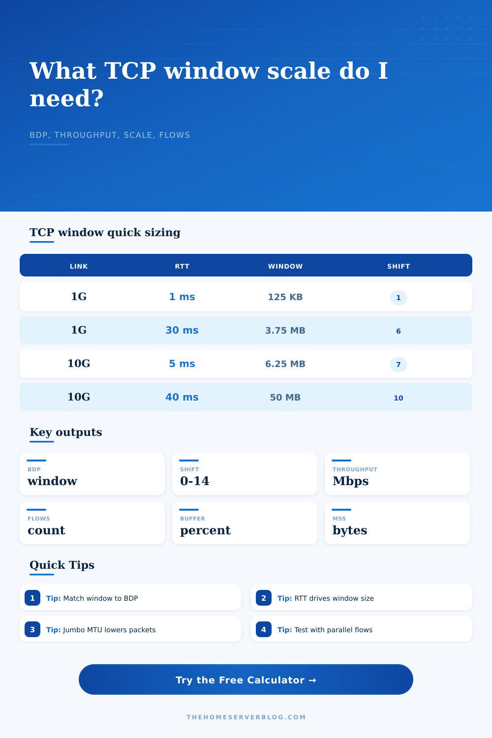
The reference table on the page spells it all out; it maps different shifts onto max window sizes for many link type. As you can see, RTT dominates. On a 1 gigabit connection, you have a small window for a one millisecond delay. If we bump that up to thirty milliseconds, then your window jumps dramaticly. This is why VPN connections seem sluggish, even when using fast internet. Encryption overhead reduce efficiency and increases latency, which means you need to increase your window to get the same throughput.
People also fail to think about protocol efficiency. No transfer in real world is perfectly efficient. There is storage protocol overhead. Headers and encryption tunnels reduces the actual payload. This allows you to tweak the efficiency percentage that the tool takes into account. For things like IPsec or WireGuard, drop it down to take into account those additional bytes per packet. That makes results far more realistic different than just a raw theoretical number.
Using Parallel Flows There’s also parallel flows. One TCP connection limit how much data can be sent over it. If the window size isn’t large enough, you can’t get a large stream flowing. Open more. That’s why tools such as iperf runs multiple threads. Each thread gets its own connection and window, splitting the load. Essentially, they are working around a limit where certain hardware can absorbs very large receive buffers in a single flow.
You don’t want to max out every single available megabit, though. You want to adjust your window to match the path. Because latency varies, it’s smart to leave yourself with a safe buffer. If you have too tight of a connection, jitter and small packet losses will freezes a connection. Having a little headroom makes for stable connections while losing only minimal speed.
And that’s the key to tuning your network, it’s not so much about chasing some number as it is about knowing how the conversation goes back-and-forth from sender to receiver. You tune your window size to match what your bandwidth and latency actualy are, and the transfer just works. That pipe fills up, the acks catch up, and you get to enjoy the speed promised on those fast links. Turns out, it’s all about having enough space in the buffer and being patient enough to let the pipe fill, you should of checked your settings first.