Conntrack Memory Calculator
Estimate Linux nf_conntrack memory for state table entries, hash buckets, NAT and accounting extensions, helper expectations, safety headroom, and clustered node counts.
Full memory breakdown
1. Per-entry memory
Entry memory starts with the measured object size, then applies NAT and accounting extension overhead.
entry RAM = entries × bytes per entry × (1 + NAT% + accounting%)
2. Bucket memory
The hash table is separate from connection objects and grows with the configured bucket count.
bucket RAM = hash buckets × bytes per bucket
3. Expectations and buffer
Helper expectations are modeled as a smaller side table, then a safety buffer is added to the whole per-node footprint.
node RAM = (entries + buckets + expectations) × (1 + buffer%)
4. Cluster total
Conntrack is local to each network namespace or node, so multiply a per-node plan by the number of nodes using it.
total RAM = RAM per node × node count
The calculator uses binary units for RAM output: 1 MiB is 1,048,576 bytes.
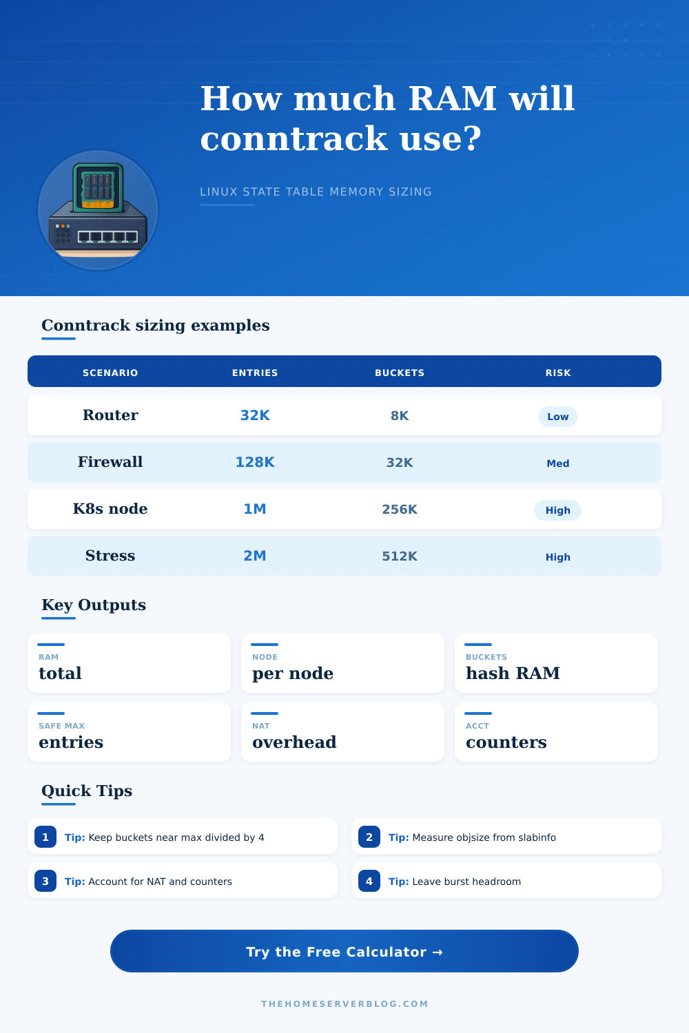
Small router
Low RAM, modest state table, few helpers, and usually no accounting. Bucket memory is tiny, but buffer matters.
Best fit: 32K to 64KNAT firewall
More short-lived flows, NAT extension overhead, and bursts from clients. Keep the bucket ratio close to kernel defaults.
Best fit: 128K to 512KContainer node
Many pods share the node state table, so conntrack memory scales with node count and east-west service churn.
Best fit: 512K to 2M| Kernel value | What it controls | Reference default | Calculator use |
|---|---|---|---|
| nf_conntrack_buckets | Hash table bucket count for connection tracking lookups. | Calculated from RAM, with documented min and max bounds. | Enter as hash buckets, then multiply by bytes per bucket. |
| nf_conntrack_max | Maximum number of connection tracking entries allowed. | Documented as bucket count × 4 on current kernel docs. | Enter as max conntrack entries for each modeled node. |
| nf_conntrack_expect_max | Maximum size of the helper expectation table. | Older kernel docs list buckets / 256 as the default. | Enter expectation table entries directly when helpers matter. |
| nf_conntrack_acct | Adds 64-bit packet and byte counters to new tracked flows. | Disabled by default in kernel documentation. | Represent this as accounting extension percent. |
| Planning value | Typical range | Why it changes | How to enter it |
|---|---|---|---|
| Base nf_conn object | 304 to 360 bytes | Kernel version, architecture, slab layout, enabled features. | Use measured objsize as bytes per entry. |
| Hash bucket storage | 8 to 16 bytes | Pointer size and list structure on 32-bit or 64-bit systems. | Use 16 bytes per bucket for conservative 64-bit sizing. |
| NAT extension | 8% to 30% | Masquerade, DNAT, SNAT, tuple manipulation, and offload metadata. | Enter the added per-entry percentage for NAT-heavy hosts. |
| Accounting counters | 0% to 12% | Packet and byte counters add memory to newly tracked flows. | Use 0 when disabled, higher when per-flow counters are on. |
| Expectation object | 128 to 256 bytes | Helpers and protocol modules create related-flow state. | This calculator uses 60% of entry bytes, minimum 128 bytes. |
| Preset | Modeled host | Why entries grow | Watch first |
|---|---|---|---|
| 512 MB Router | Small OpenWrt-style edge router | Browsers, phones, package updates, and DNS churn. | Keep memory footprint below small-device free RAM. |
| 2 GB Home Firewall | x86 firewall, pf-style appliance, or Linux gateway | Client NAT, VPN users, media services, and bursts. | Max-to-bucket ratio and NAT extension overhead. |
| Kubernetes Worker | Worker node with pod networking and service NAT | Pod fan-out, node-local services, short-lived API calls. | Per-node memory multiplied by worker count. |
| Proxmox NAT Host | Hypervisor with lab VMs behind masquerade | Many guest operating systems sharing one state table. | VM bursts during updates and backup windows. |
| Lab Stress Test | Intentional high-connection test box | Large entry count, long buckets, and all overheads enabled. | Slab growth, CPU lookup cost, and reclaim pressure. |
| Max entries / buckets | Bucket pressure | Meaning | Practical action |
|---|---|---|---|
| Up to 4x | Comfortable | Matches the commonly documented default ratio. | Good starting point for routers and firewalls. |
| 4x to 8x | Watch | Memory stays low, but average chains get longer. | Increase buckets if CPU lookup cost rises. |
| 8x to 12x | Tight | High state count packed into a smaller hash table. | Tune hashsize along with nf_conntrack_max. |
| Above 12x | High risk | May trade a little RAM for noticeably longer lookups. | Rebalance buckets before raising max further. |
When the connection tracking table fill up, you’ll see a warning in kernel that it’s dropping packets. Your network will become sluggish or even time out, something that didn’t happen before. To instantly eliminate these warnings, increase the `nf_conntrack_max`. But doing so overlooks memory cost associated with every tracked connection. Each one consumes memory, and soon those costs adds up.
By simply inputting how many buckets you want and how many entries they will contain, calculator does all of the work for you. It begins with one tracked flow and its base object size. That’s anywhere from three hundred to three hundred sixty bytes on current kernels. Multiply that by tens of thousands of connection, and it uses a lot of RAM. You can modify that baseline according to your kernel version. If you have something different than the generic average, then planning based off that average will be inaccurate.
How to Plan Your Network Memory
These connections is stored via pointers in buckets within the hash table. Increasing your maximum number of entries but not proportionally increasing the number of buckets result in long chains within the hash table that require CPU to walk more pointers on each lookup. This waste processing cycles and increases latency. There is even a field in the calculator to account for bucket overhead so you can understand just how much those pointers cost. Maintaining a ratio of about four to one between buckets and your maximum number of entries improve lookup speed while using as little memory as possible.
Each connection is also bigger when there are extensions like accounting, hiding, NAT etc. There may be extension to account bytes per flow, which adds another layer of complexity. They vary with the nature of your traffic. You can enter the overhead percentages on these feature in the tool. At one extreme, if it’s a pure routing node, it could disregard the overhead, whereas at the other end, a gateway doing internal network address translation would have more overhead per entry.
Planning ahead avoids being surprised when memory runs out during the busy period. In a Kubernetes cluster, every worker node has its own state table. It’s not as simple as dividing your cluster’s total amount of RAM across some randomly chosen number and calling it “the memory available for connections.” The calculator assumes you have some amount of nodes (because otherwise the entire point is moot), then multiplies the per-node footprint by that number. This give you an idea of what your aggregate consumption is likely to be. This allows capacity planners to provide enough infrastructure without providing too little. This is important if you are starting up new services with lots of connection churn.
These helper expectations cause memory costs, but the memory cost is reduced nowadays when the helpers is typically turned off due to security concerns. In case of FTP/SIP helpers, expect these tables as well. The safety buffer input provides extra space for slab allocator overhead and bursts in traffic pattern. This will also allow for uneven bucket distribution. A rule of thumb would be to keep at least one quarter or even more as a safety buffer against transient spikes pushing you over the edge towards packet drops.
Memory pressure in kernel land isn’t linear. More often it’s sudden with noticeable slowness rather than slow and getting slower over time. Knowing what use that memory helps you make an informed choice. You can decide whether to add RAM, adjust your NAT rules, or limit your number of concurrent connections. Your goal is stability, not overprovisioning.
Stateful networking carries an expense and we should respect our hardware limitations. We must weigh our RAM supply vs. Our CPU efficiency. Every configuration decision affect this tradeoff. By breaking into buckets, entries, extensions, and buffers, we transition from guessing to engineering with understanding. This transforms what was once a possible outage situation into a solvable capacity issue.
Your network runs smoothly under load and you never see that dreaded packet drop warning again. Actualy, it helps ensure your networks is always stable. You should of checked this earlier.