Database capacity and retention planning
Database Growth Projection Calculator
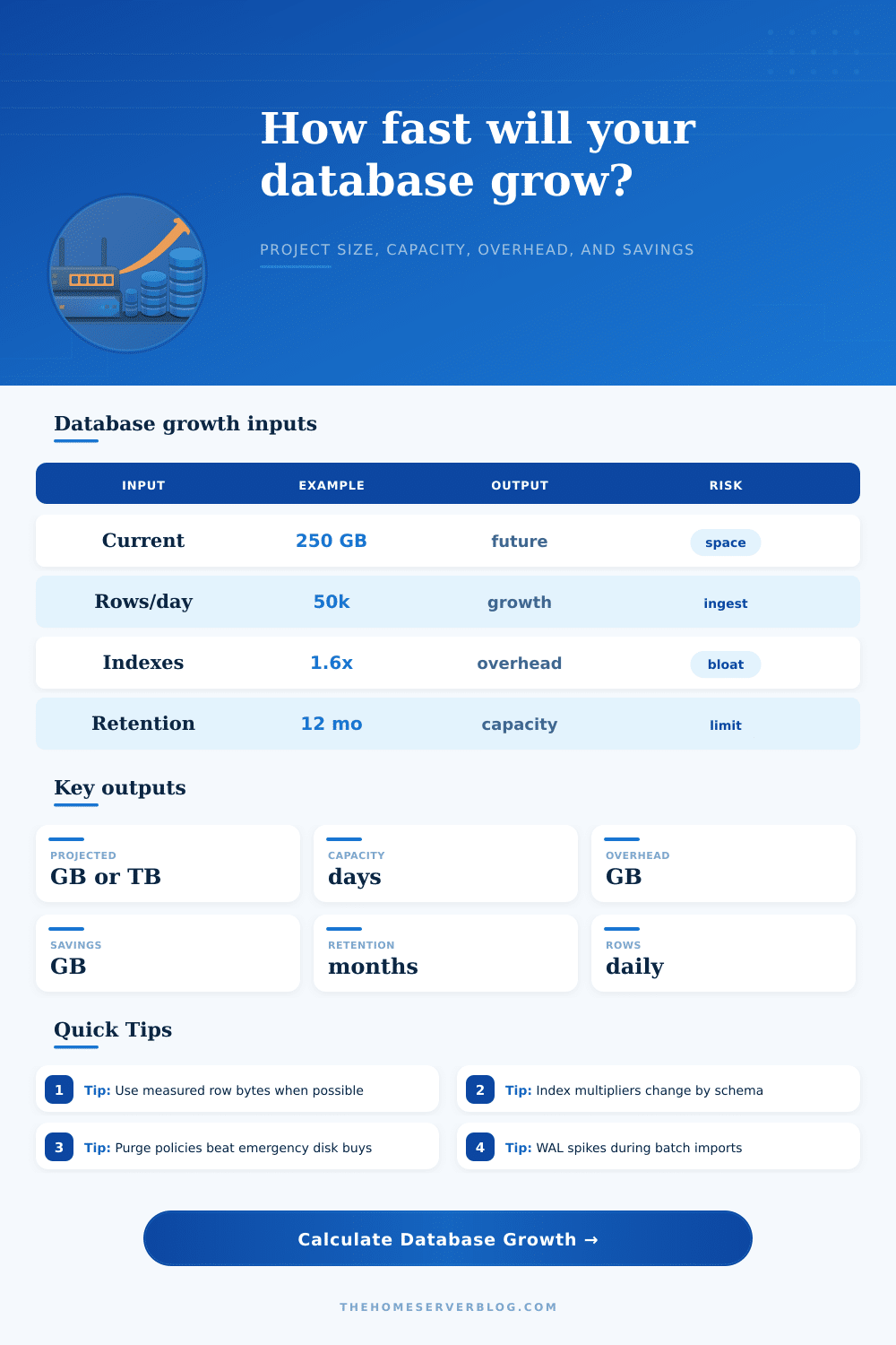
Estimate database size at the retention horizon, days until the capacity limit, index and WAL or binlog overhead, and storage saved by purge, archive, and compression policies.
Growth formula breakdown
Capacity and overhead reading
| Checkpoint | Raw added | Retained compressed rows | Index + log overhead | Total projected size | Capacity used |
|---|---|---|---|---|---|
| Month 1 | 0 GB | 0 GB | 0 GB | 0 GB | 0% |
PostgreSQL OLTP
Index range: 1.3x to 2.2x. WAL can spike during bulk writes, index builds, autovacuum churn, and logical replication.
MySQL InnoDB
Index range: 1.2x to 2.0x. Secondary indexes include the primary key, so wide clustered keys increase growth.
SQL Server
Index range: 1.4x to 2.5x. Nonclustered indexes, row versioning, and log backup cadence affect capacity planning.
SQLite Edge Store
Index range: 1.1x to 1.7x. WAL mode and vacuum behavior matter on small disks and embedded appliances.
Time-Series Engine
Index range: 1.1x to 1.6x. Compression, chunk retention, and downsampling usually dominate long-term size.
Object Archive Tier
Index range: 1.0x to 1.2x. Best used after partition detach, cold export, or immutable audit retention rules.
| Workload | Common rows/day | Average row size | Index multiplier | Planning note |
|---|---|---|---|---|
| Home Assistant Recorder | 20,000 to 500,000 | 0.2 to 1.2 KB | 1.2x to 1.7x | Retention and entity exclusions usually matter more than raw row size. |
| WordPress Content DB | 50 to 5,000 | 2 to 30 KB | 1.3x to 2.0x | Post meta and plugin tables can outweigh posts and comments. |
| WooCommerce Orders | 100 to 25,000 | 4 to 40 KB | 1.5x to 2.5x | Order meta, sessions, webhooks, and analytics tables need separate checks. |
| Time-Series Metrics | 500,000 to 100,000,000 | 0.05 to 0.8 KB | 1.1x to 1.5x | Chunk compression and downsampling decide whether the trend is manageable. |
| Audit Log Warehouse | 100,000 to 20,000,000 | 0.5 to 8 KB | 1.2x to 1.8x | Legal retention can be long, so archive tiering should be modeled early. |
| Formula piece | Calculator method | Why it matters | Input to tune |
|---|---|---|---|
| Raw daily ingest | rows/day x average row KB / 1,048,576 | Converts logical rows into GB before retention policies. | Rows/day and average row KB |
| Compounded ingest | Monthly growth changes the row rate across the horizon. | A small percentage compounds quickly in tenant or device workloads. | Monthly growth % |
| Retained row storage | Raw added x (1 - purge rate) x (1 - compression) | Shows the live primary footprint after cold data movement. | Purge/archive and compression % |
| Index overhead | Retained compressed rows x (index multiplier - 1) | Wide secondary indexes can make row growth look deceptively small. | Index multiplier |
| Log overhead | Retained compressed rows x WAL/binlog overhead % | Captures retained log, CDC, replica, and recovery storage allowance. | WAL/binlog overhead % |
| Pattern | Typical retention | Purge or archive rate | Compression fit | Capacity signal |
|---|---|---|---|---|
| Operational OLTP | 3 to 18 months | 10% to 60% | Low to moderate | Capacity should stay below 75% after peak season. |
| Append-only ledger | 36 months or longer | 0% to 20% | Moderate | Plan partitions because deletes are often restricted. |
| Metrics and sensor data | 7 days to 13 months | 40% to 95% | High | Downsampling changes the slope more than indexes do. |
| Audit and access logs | 12 to 84 months | 30% to 90% | High | Archive search requirements determine how cold data is stored. |
| Collaboration metadata | 12 to 36 months | 5% to 40% | Low to moderate | Soft deletes and history tables can hide retained growth. |
| Overhead source | Low estimate | Typical estimate | High estimate | What to inspect |
|---|---|---|---|---|
| Secondary indexes | 10% to 40% | 40% to 120% | 120%+ | Index count, composite keys, included columns, duplicate indexes. |
| WAL or binlog retention | 5% to 15% | 15% to 45% | 45%+ | Backup cadence, replica lag, CDC slots, batch import windows. |
| MVCC and bloat | 5% to 15% | 15% to 35% | 35%+ | Vacuum health, update rate, dead tuples, page splits. |
| Partition metadata | Small | Moderate | Large at scale | Partition count, catalog size, detached archive tables. |
| Compression savings | 5% to 15% | 15% to 50% | 50%+ | Repeated text, JSON, time-series chunks, columnar exports. |
If you’ve ever woken up to an after-hours notification that your disk space has spiked over eighty percent, you know how it goes: Panic! Search around for some dead indexes! Scale up production traffic! The problem isn’t typically that there’s so much more data; its that you didn’t anticipate how much storage would be required over time. Instead of thinking of your database as a dynamic system, you might think of it like a fixed bucket of capacity. Each new row take up space in transaction logs and in indexes, space that adds weight without adding value. Missing this can cost dearly when you buy hardware on an emergency basis which comes with both downtime and panic-premiums.
With those inputs, the calculator shown above will compute them for you. It doesn’t just tally up the bytes. It accounts for the hidden cost of indexes not listed in the main table. It also models how raw data will build up over time. By asking you to specify an index multiplier, you’re recognizing that secondary indexes takes up space relative to their keys. An index multiplier of 1.5 signifies that indexes add fifty percent overhead to the stored row data. Your mileage may vary based off the nature of your schema design. If you’ve designed a narrow key on your primary table and are using a time-series engine, this number could be closer to 1.1. If your schema is wide with a composite key, such as an elaborate e-commerce system, it could creep towards two. The accuracy of this coefficient is the difference between having six months of runway versus storage crisis by next quarter.
How to Calculate Your Database Storage Needs
The retention policy is where all of the assumptions break down, as everyone assumes that they’re going to retain everything “forever.” To illustrate the impact of actively managing your datas lifecycle, the tool allows you to test different purge rates along with how much compression can save you. Downsampling minute-by-minute sensor data or archiving old audit logs isn’t just good housekeeping; it directly impacts your storage costs. You may simply assume that deleting 10 percent of your rows will save you 10 percent space, but reality is more messy. Transaction log retention and index fragmentation often weaken or delay these savings until you run a rebuild/ vacuum phase. The calculator accounts for those overheads so you don’t overestimate how much immediate relief a purge job provides you.
Think about two types of databases: an operational database versus an analytical warehouse. While an OLTP system needs fast queries (i.e. An OLTP system needs fast queries with low latency. This makes it rely on heavy indexing, which eats up disk space quickly. To conserve space for large batch loads, a data warehouse may not heavily index and just store raw JSON payloads instead. That architecture tug-of-war should be reflected in your forecasting plan.
For example, if you’re providing a SaaS app and adding more tenants every month, the growth rate as a percentage per month is key. Four percent per month may sound reasonable, but when compounded over a dozen months, that’s a lot of rows being ingested. The tool takes into account that compounding factor and shows you the curve ahead of time so you don’t hit your capacity ceiling.
Cloud providers has made provisioning easy; making scaling appear smooth; therefore we tend to think of our storage capacity as unlimited. But automation only goes so far, and rapidly increasing your instances class just to accommodate idle historical data will break the bank. Planning ahead turns an emergency into a scheduled maintenance period. To find what works best for you, try testing different retention times in the tool. This will help you see how fast you reach your limit when using more permissive storage versus more aggressive archiving. From there you’ll be able to make an educated guess of when you need to optimize your schema, add tiered storage solutions, etc, before your disk fills up.
In the end, what we’re aiming for here is a sense of your future infrastructure requirements. If you have an accurate handle on your database growth (after accounting for the overhead that hides in plain sight) then you’ll be able to predict growth as well. From there, once you understand the interplay between row size, index multipliers, and log retention, you’re in control, not beholden to whatever the storage meter says when it’s time to pay up or go down.
It’s just basic math, but having the discipline to model this in advance would of helped you separate the stable system from one always teetering on the edge. With today’s metrics, plug them into the formula and let the forecast play out. Then you’ll have better visibility into what you need for the next period so you can sleep more soundly.