Databricks Cluster Size Calculator
Plan Databricks workers, driver size, vCPU and RAM pool, shuffle storage, autoscale range, concurrency, and Photon fit for Spark jobs, SQL workloads, ML, and streaming.
Recommended Databricks Cluster Shape
| Mode | Best fit | Sizing emphasis | Autoscale note |
|---|---|---|---|
| Job cluster | Scheduled ETL, Delta merges, repeatable pipelines | Duration target, shuffle spill, predictable worker max | Start near calculated min; cap at SLA peak |
| All-purpose shared | Notebook teams and mixed exploratory work | Concurrency, driver memory, idle floor, queue tolerance | Higher minimum avoids cold ramp during collaboration |
| Single-user | Debugging, model iteration, isolated development | Responsive driver, moderate workers, fast task feedback | Keep range narrow unless data size is volatile |
| SQL warehouse style | Dashboard bursts and SQL-heavy analytics | Photon, concurrency, short query latency, cache reuse | Use a wider max for bursty dashboard traffic |
| Worker class label | vCPU | RAM | Typical use |
|---|---|---|---|
| Standard 8 | 8 | 32 GB | Small jobs, testing, light notebooks |
| Standard 16 | 16 | 64 GB | Balanced ETL, Delta write workloads |
| Memory 16 | 16 | 128 GB | Wide rows, feature builds, joins with skew |
| Memory 32 | 32 | 256 GB | Large shuffles, ML preparation, high-cardinality aggregation |
| Compute 16 | 16 | 32 GB | CPU-heavy transforms with low memory pressure |
| Photon-ready 16 | 16 | 64 GB | SQL, Delta scans, dashboard acceleration |
| Workload type | Starting multiplier | Memory note | Photon fit |
|---|---|---|---|
| Batch ETL | 1.0x | Balanced RAM per core | Helpful for Delta operations |
| SQL analytics | 0.75x with Photon | Cache and concurrency matter | Strong fit |
| ML feature engineering | 1.25x | Favor memory classes | Depends on transforms |
| Structured streaming | 1.15x | Keep steady-state headroom | Usually secondary |
| Large shuffle | 1.45x | Spill and skew dominate | Useful for SQL joins |
When your Spark job runs for three hours and is just 20% complete, there’s typically one reason: the cluster was set up based off data volume rather than computation shape. So naturaly, you’d add more workers to accelerate that run. You will eventually reach a limit where adding nodes increase network traffic without providing enough additional processing power. Shuffle spills and driver memory pressure becomes the bottlenecks rather than CPU wait time. The calculator shows these tradeoffs, but understanding what goes into them is difference between having a real pipeline and just getting lucky.
Don’t just look at gigabytes; look at type of workload. Is it an ETL job? If yes, then it’s probably moving data in a linear fashion and would benefit from more balanced memory/CPU resources. Is it a SQL analytics workload? If yes, then it’s likely executing queries concurrently and using cache, and would thrive with more RAM.
How to Fix Slow Spark Jobs
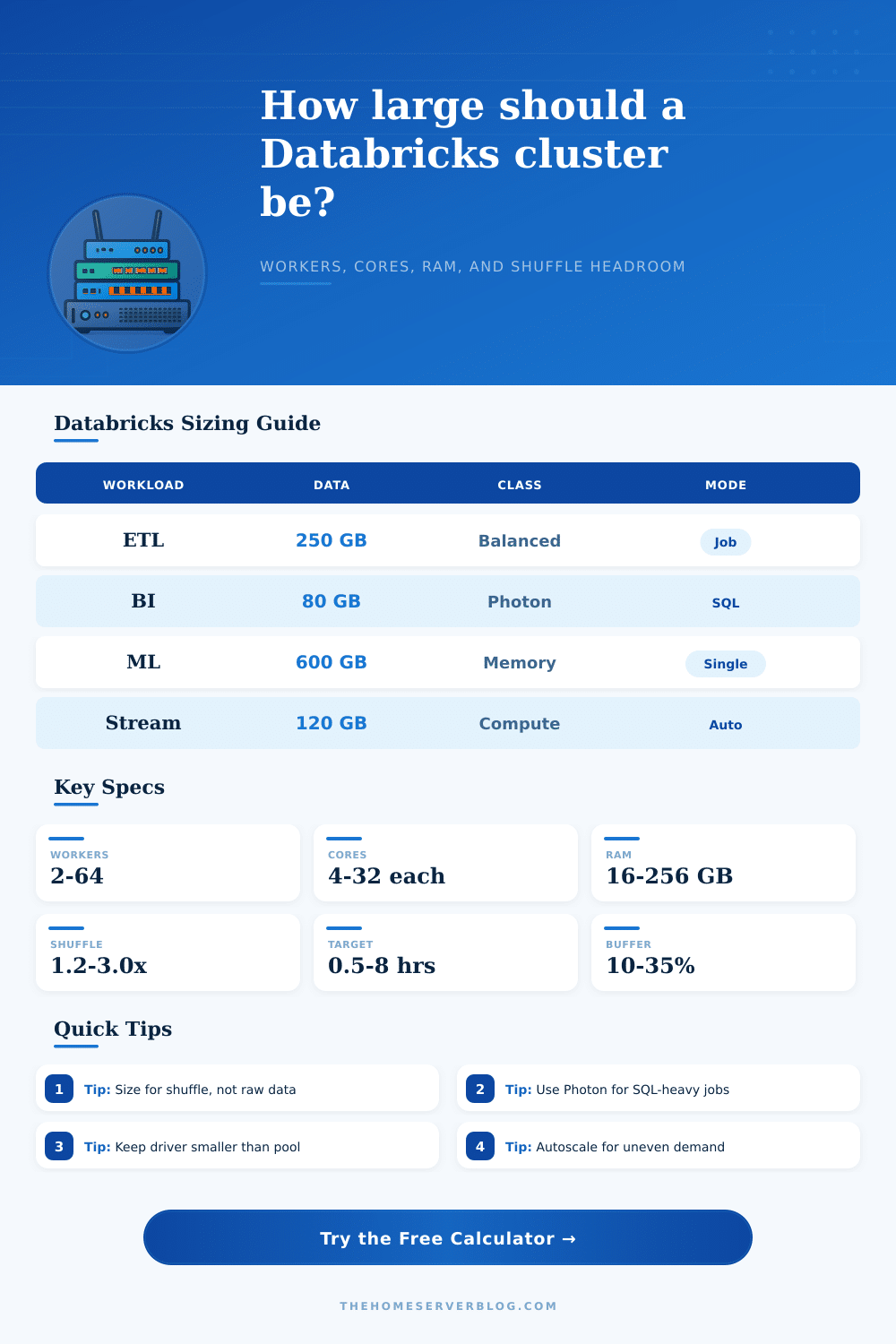
The cost to move data around over network partitions is underappreciated by most teams, and that’s precisely why there’s a shuffle multiplier input. Take, for example, a big join operation between two massive tables colliding in memory. Unless your worker nodes has sufficient RAM to store those partitioned chunk, they dump them to disk instead. Even with a ton of cores available, this cause your job to slow down dramatically due to much slower memory access different than disk I/O.
With the tool, you can estimate required headroom in local storage before that happens; you input a multiplier based on the heavyness of the transformation, and it will automatically adjust the recommendation for an appropriate instance class. That way, you avoid common mistake of going cheap on compute-optimized nodes only to run out of memory midway into your job.
The autoscaling settings are an afterthought (but so important). They’re what set floor on your cost efficiency. If you set the minimum worker count too low, then each new query incurs a cold start penalty while servers spin up. That latency kills dashboard responsiveness and frustrates data analyst trying to get answers. But if you set max too high, then you invite waste at quiet hours with nobody running queries. You want right range to keep a warm pool of workers ready for burst traffic but not waste money by keeping all that expensive hardware idle overnight. It’s a balancing act, between your budget and your need for speed, that depends entirely on usage patterns.
Equal consideration should of given to driver configuration, which directs everything. Scheduling becomes a bottleneck when you have a tiny driver controlling a huge number of workers. Thousands of executor need their metadata, their tasks, and their results tracked by the driver at all times. When this falls behind, the workers waits idly for direction. Ideally, your driver is sized based on how hard the job is rather than being small simply to save a buck. You don’t want the head node slowed down by coordinating tasks. This is especially true when doing machine learning feature engineering or complex Delta merges.
The same is true of SQL, photon acceleration basically vectorizes operations and eliminates JVM overhead from the equation. Enabling this will change resource profile, as engine can execute more efficiently per core. What does that mean? Either get away with fewer workers executing same queries, or run much more concurrent traffic on the same hardware. It doesn’t make it a magic button, but it does optimize the execution path in ways that makes you reconsider your instance selection.
The last step is to benchmark. No moddern model exactly matches the nuance of your data distribution. A skewed key might overwhelm one partition, breaking even well-sized clusters. Treat these estimates as your initial hypothesis and test it against real-world Spark UI metrics: how much did tasks spill? How long they take? It’s an iterative tuning process, but making the right architectural assumptions will save you weeks of debug time down the line. Nail the foundation; polish the details.