Fiber Propagation Delay Calculator
Estimate one-way fiber latency, round-trip delay, effective optical path length, and delay per kilometer from refractive index, velocity factor, slack, and route factors.
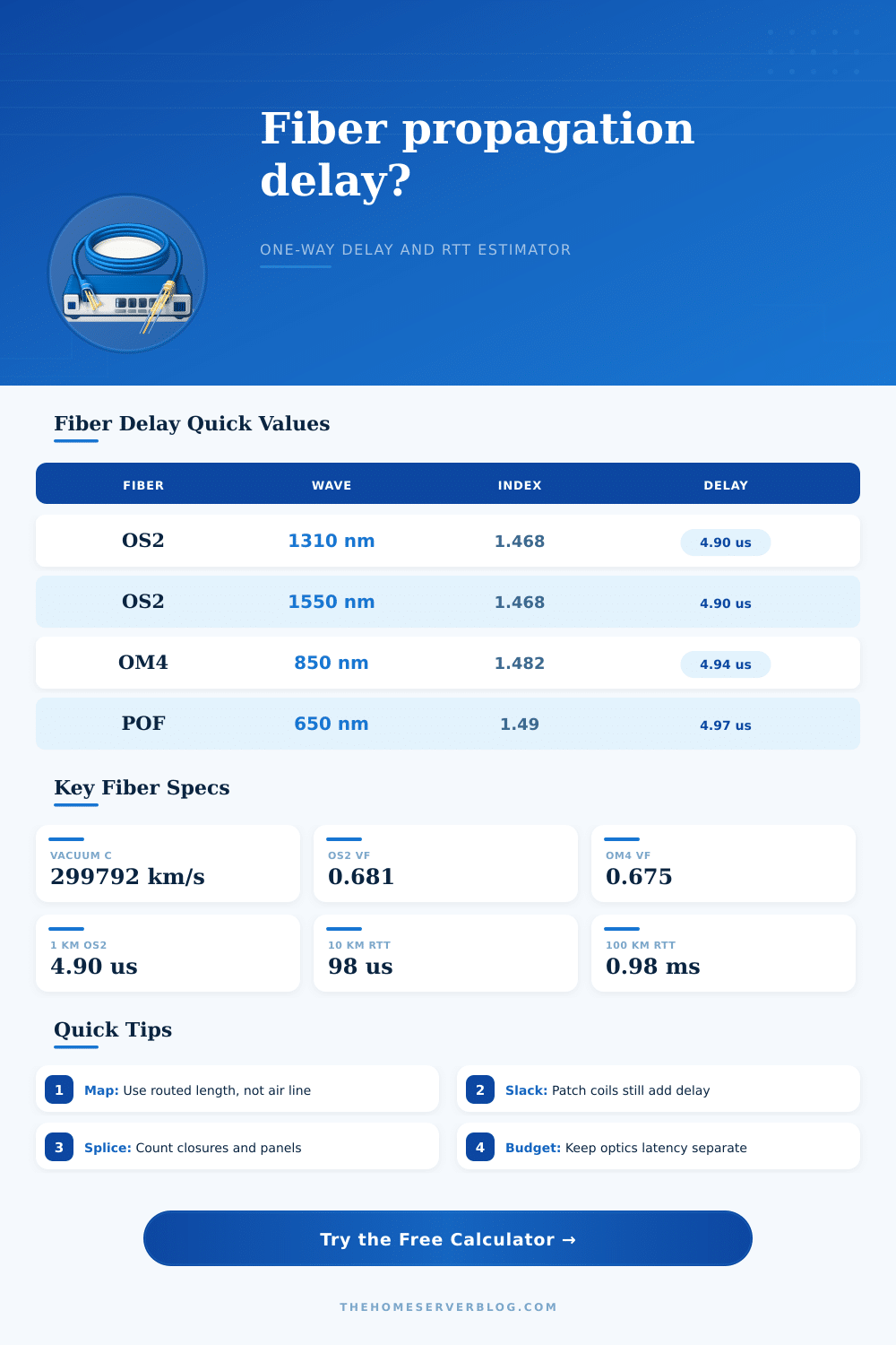
| Fiber profile | Wavelength | Typical group index | Approx delay |
|---|---|---|---|
| OS2 singlemode | 1310 nm | 1.4677 | 4.90 us/km |
| OS2 singlemode | 1550 nm | 1.4682 | 4.90 us/km |
| OM3 multimode | 850 nm | 1.4820 | 4.94 us/km |
| OM4 multimode | 850 nm | 1.4815 | 4.94 us/km |
| Bend-insensitive SMF | 1550 nm | 1.4680 | 4.90 us/km |
| Plastic optical fiber | 650 nm | 1.4900 | 4.97 us/km |
| Scenario | Nominal length | Fiber type | Planning note |
|---|---|---|---|
| Rack patch OS2 | 30 m | OS2 1310 nm | Patch slack dominates the small delay. |
| Room OM4 trunk | 75 m | OM4 850 nm | Good for short multimode switch uplinks. |
| House backbone | 120 m | OS2 1310 nm | Small RTT, but include tray and wall slack. |
| Campus OS2 | 2.5 km | OS2 1550 nm | Routing factor matters more than patch cords. |
| Regional WAN | 85 km | OS2 1550 nm | Fiber path sets a visible latency floor. |
| Effective length | One-way OS2 | Fiber RTT | Typical use |
|---|---|---|---|
| 10 m | 0.049 us | 0.098 us | Same rack or adjacent rack |
| 100 m | 0.49 us | 0.98 us | Home, lab, or small building |
| 1 km | 4.90 us | 9.79 us | Campus or neighborhood run |
| 10 km | 49.0 us | 98.0 us | Metro access path |
| 100 km | 0.49 ms | 0.98 ms | Regional fiber span |
| Reference | Value | Meaning | Calculator use |
|---|---|---|---|
| Speed of light | 299,792,458 m/s | Vacuum reference speed | Multiplied by velocity factor |
| Velocity factor | 1 / group index | Fraction of vacuum speed | Sets propagation speed |
| Route factor | 0 to 80 percent | Extra path for ducts and risers | Added to base cable length |
| Patch slack | Per end | Service loops and patch coils | Added twice by default |
| RTT | 2 x one-way | Fiber-only round trip | Compared with budget |
The spreadsheet reads like a dream. The ping from Chicago to New York is low; the database in one city speak fluently to the server in the other. Throughput is high, so you deploy application with confidence. But as number of users scales up, you realize there’s a problem. Not with bandwidth. With light speed. Or should I say the lack of it?
Fiber propagation delay slow down every photon that gets trapped in silica glass. This delay is hard floor on network latency and no amount of protocol optimization or buffering can erase it. When you understand this physics constraint, you’re able to design for performance with precision, not guesswork.
Understanding Fiber Delay
The calculator above will do the math for you. But knowing how numbers work is more valuable then the number itself. Most planners model fiber as a straight line between two points where distance equals travel time. In the real world, it’s never a straight shot. Route factors include tray meander, duct bend and riser climb. And there is patch slack in coils at each termination point. It’s not just an inventory thing; it makes the delay much worse. On a floor plan, that thirty-meter patch cord may appear to be short in a rack, but once you add in connector panels and service loop, the optical path can get much longer. All of that additional glass add microseconds that compound over large networks.
And that brings us to the invisible governor: refractive index. This tell us how much light slows down compared to vacuum speed. At normal telecom wavelengths, single mode fiber (e.g., OS2) tend to be somewhere around 1.468. Some multimodes may be higher, thus pushing delay up slightly. The tool will make this conversion for you from refractive index to velocity factor or vice versa, whichever you prefer.
Velocity factor is just a number representing how many times faster than the speed of light your signal is traveling, if only it were. See a 0.68? Well then your signal are moving along at approximately six-eighty percent of theoretical top speed. Not a flaw. Not a problem. Just material science. Light interacts with structure and mass. And silica glass does have some structure and mass. This is spelled out on the page with a handy table of reference material for common fiber types and their wavelength ranges.
For common single-mode (OS2) fiber at two popular bands, 1310 nanometers and 1550 nanometers, the delay are nearly identical. Latency budget-wise this difference is negligible although loss of power differs between bands. That’s not so much the case for plastic optical fiber. Its higher refractive index (around 1.49) cause slightly increased delay per kilometer. At short range (say audio link or home automation) that fraction of a microsecond won’t make any difference. Every nanosecond makes a difference when you’re doing something like distributed database consistency checks or high frequency trading.
Fiber latency and network lag gets confused all of the time. They’re different things. Fiber latency is purely a function off physics. It’s the time it takes for that first photon to go from point A to point B. That’s called propagation delay. Other factors like queueing delay, packet serialization, protocol overhead, switch processing… All of those adds up to what we call network lag. The fiber portion of the calculator removes all of that so you can actualy see the baseline.
If you find that the actual round-trip time you measure is much larger than this number, you have a pretty good idea where the issue lies. It isn’t on the glass; it’s either an issue with the software stack or the electronics. Always allow for the unknown when building a metro loop or campus backbone. Closures bulge with extra fiber needed for maintenance. Ducts move around. That service loop is just dragging down your latency budget. You can enter number of splices in the tool as well as how much slack allowance per splice. Do so. Designing for a marginally longer path beats finding out at commissioning that your route factor was too optimistic. Go conservative now, save some headaches later.
You should of gone conservative from the start. Finally, remember that while light travels quickly, it doesn’t travel instantly. The difference between amateur installs and professional engineering is understanding the physics of fiber optics in a microsecond-driven world where competitive advantage hinges on microseconds. There’s no cheating the speed of light; however, there are ways to plan for it. When you understand exactly what your cable plant adds by way of delay, you’re able to make educated hardware-placement and layout decisions. This transforms an abstract constraint into a manageable variable. That kind of clarity is worth its weight in gold come go-livig day.