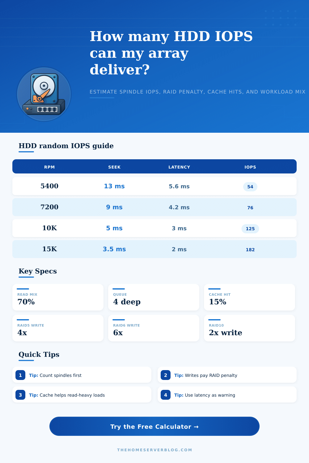
Hard Disk IOPS Calculator
Estimate HDD spindle IOPS from RPM, seek time, queue depth, RAID level, cache hit rate, and random versus sequential workload blend.
| HDD class | Average seek | Average rotation | Random IOPS estimate |
|---|---|---|---|
| 5400 RPM archive or quiet NAS | 12 to 14 ms | 5.56 ms | 50 to 58 IOPS |
| 5900 RPM low power desktop | 11 to 13 ms | 5.08 ms | 55 to 62 IOPS |
| 7200 RPM NAS or enterprise SATA | 8 to 10 ms | 4.17 ms | 70 to 82 IOPS |
| 10K SAS performance HDD | 4.5 to 5.5 ms | 3.00 ms | 118 to 133 IOPS |
| 15K SAS legacy performance HDD | 3.0 to 4.0 ms | 2.00 ms | 167 to 200 IOPS |
| Layout | Read scaling | Small write penalty | Best home server fit |
|---|---|---|---|
| Single disk or JBOD spread | Up to all disks if balanced | 1 physical I/O | Cold media, backups, scratch disks |
| RAID 0 stripe | All spindles | 1 physical I/O | Temporary fast space with no redundancy |
| RAID 1 mirror | Both disks can read | 2 physical I/Os | Boot pools and small mirrored NAS |
| RAID 5 parity | Most spindles can read | 4 physical I/Os | Read-heavy four to eight disk pools |
| RAID 6 dual parity | Most spindles can read | 6 physical I/Os | Larger HDD arrays and safer rebuilds |
| RAID 10 mirror stripe | All spindles can read | 2 physical I/Os | VM storage and write-heavy home labs |
| Workload type | Random share | Read mix | Queue depth note |
|---|---|---|---|
| Media streaming NAS | 10% to 30% | 80% to 95% | Low queue depth, mostly sequential reads |
| Photo library and file shares | 40% to 60% | 65% to 85% | Short bursts from many small files |
| VM datastore on HDD | 75% to 95% | 55% to 75% | Queue depth matters but latency rises |
| Surveillance recording | 5% to 20% | 5% to 25% | Sequential writes dominate |
| Backup target | 15% to 35% | 10% to 35% | Mostly large write streams |
| Scenario | Spindles | Typical layout | Practical note |
|---|---|---|---|
| Two-bay mirrored NAS | 2 | RAID 1 or ZFS mirror | Good reads, single-disk write feel |
| Four-bay media box | 4 | RAID 5 or RAIDZ1 | Strong reads, parity write penalty |
| Six-disk VM lab | 6 | RAID 10 or mirrored vdevs | Lower write penalty for small random I/O |
| Eight-disk backup shelf | 8 | RAID 6 or RAIDZ2 | Safer rebuilds with slower random writes |
| Twelve-disk archive pool | 12 | Dual parity groups | Plan around rebuild load and scrub windows |
Sure, you bought those hard drives because they held so much stuff. They was supposed to hold three hundred gigs of old photos, or maybe five terabytes of video. That’s why you bought them, that was the selling point.
But then you go to run a virtual machine off that array, and holy crap, does it grind to a halt. It’s not because there isn’t enough space, it’s because there aren’t enough IOPS (input operations per second). And unlike space, IOPS is tiny on spinning rust versus flash storage. And that IOPS number dictates whether your server feel snappy or sluggish.
Why Hard Drives Are Slow With Random Data
But real world physics apply to a hard disk; every random read has to move the actuator arm to the new track, then wait until the platter rotates back around so it can reach actual data. The sum of seek time + rotational latency = service time. A typical 7200 RPM drive could take up to ten milliseconds to locate a single little block of data. Do the math, you’ll see that at most your disk will be able to handle about one hundred operations per second before it’s fully saturated. Most folks dramatically overestimate what their few random writes does with that budget.
There’s another sneaky tax on this performance: RAID levels. While adding redundancy with parity protection is great, in a RAID five configuration, it means a single small write can require quadruple the effort. If your RAID level is five, then a little tiny write can become four physical writes (read old data, read old parity, calculate new parity, write new data). This is a killer of throughput.
When you pick out your layout, the calculator above will tell you exactly how many spindles you need to cover this overhead. Ignore the overhead and you’ll purchase storage that may look big but will perform poor under a load.
Hard drives are terrible at handling multiple requests simultaneously; that’s where queue depth comes into play. The more commands it receives from your workload in parallel, the longer it take to switch between them and the less time it has working; this is why the queue will cause latency spikes. A small queue maintains consistent latency for random workloads (think: virtual machines or databases). Higher queues, meanwhile, maintain throughput for sequential data streams such as media playback. The catch: know what kind of workload you’ve got. Table on the page shows this clearly by scenario. Backup target vs. NAS).
Read-heavy situations will get a boost from cache hits: The IOPS cost will drop nearly to zero if the controller or operating system can serve the request directly from memory (RAM) vs. The system has to spin up the disk. You’ll see this matter most in repeated access patterns. Caching is huge for a photo library that’s going to be viewed over and over again; it doesn’t do much for a surveillance camera, which writes new unique video frames every second. The calculator lets you tweak the hit rate to account for this, and it gives more realistic picture of how the host will perform vs. The raw limits of those spindles.
With sequential workloads, it’s a different story. Because data comes in big blocks, there isn’t much seeking for the drive. It simply continues writing at full speed until it has filled its cylinder. So while hard drives struggle with low IOPS, they shine during sequential workloads. You’re transferring large files and your workload is largely sequential, so you don’t care about operations per second; rather, you care about megabytes per second. These two mixed together make a complicated blend. Separating the random IOPS burden from the sequential throughput help you see which factor is limiting your performance.
There are always trade offs when building an HDD array. You must pick two from density, redundancy, or speed. For example, if you set up a RAID ten mirror stripe, you get great read performance and ok write performance, but you lose half of the capacity due to mirroring. On the other hand, if you use a RAID six array, you get double parity safety on a large array, but small writes will be painfully slow. The math doesn’t lie; you don’t get something for nothing. You should of known that.
You don’t want a theoretical max; you just want something you know is sustainable. You want some headroom so that when people do spike, there’s no buildup in the queue. Latency beyond twenty milliseconds starts getting perceptible to the user. If you understand the RAID penalties and the mechanical constraints of the disks, you can properly size an array for your workload rather than going purely based off a capacity basis. Make sure your data’s pattern matches how the disk work.