CIDR route summarization planner
Prefix Aggregation Calculator
Estimate how contiguous IPv4 or IPv6 prefixes collapse into CIDR summaries, then compare target aggregate size, exception routes, route limits, utilization, growth buffer, and wasted address space.
How the CIDR model works
The calculator first builds the exact minimal CIDR cover for a contiguous run by repeatedly taking the largest power-of-two block. It then compares that exact cover with the requested target summary prefix.
Aggregation breakdown
| Original blocks | Start prefix | Single summary | Capacity effect |
|---|---|---|---|
| 2 contiguous blocks | /24 or /48 | /23 or /47 | No wasted space when aligned on the parent boundary. |
| 4 contiguous blocks | /24 or /48 | /22 or /46 | Classic one-step route reduction for powers of two. |
| 8 contiguous blocks | /24 or /48 | /21 or /45 | Useful for branches, sites, POPs, and routed VLAN groups. |
| 16 contiguous blocks | /24 or /64 | /20 or /60 | Often used for Kubernetes pools and IPv6 subnet bundles. |
| Scenario | Starting routes | Aggregate style | Planning note |
|---|---|---|---|
| Four /24 to /22 | 4 IPv4 routes | One /22 | Clean if the first /24 is aligned to a /22 boundary. |
| Eight /48 IPv6 Sites | 8 IPv6 routes | One /45 | Summarizes site assignments while leaving huge subnet capacity. |
| Branch /27 Blocks | 12 IPv4 routes | Target /23 | May intentionally cover unused adjacent /27 space. |
| Anycast POP Prefixes | 24 routes | Several /21s | Exceptions can preserve traffic engineering per POP. |
| Address family | Bit width | Common start | Useful capacity view |
|---|---|---|---|
| IPv4 | 32 bits | /24 customer or VLAN | Exact address count, such as 256 addresses per /24. |
| IPv4 | 32 bits | /27 service block | Thirty-two addresses per block before host reservations. |
| IPv6 | 128 bits | /48 site assignment | Count addresses and /64 LAN units separately. |
| IPv6 | 128 bits | /56 small site | Shows how many /64s fit the planned summary. |
| Exception type | Why it exists | Route impact | When to remove |
|---|---|---|---|
| Migration more-specific | Move one VLAN, VPC, or tenant first | Adds one route per exception | After all traffic uses the aggregate cleanly. |
| Traffic engineering | Prefer a different uplink or region | Preserves extra control at route scale cost | When policy can move to communities or metrics. |
| Firewall separation | Keep DMZ, NAT, or provider edge explicit | Consumes route max headroom | When policy is enforced below the routing layer. |
| Temporary leak | Advertise one child during cutover | May defeat some aggregation savings | After monitoring confirms parent reachability. |
Prefix aggregation is a jigsaw puzzle for network engineers: How neatly can we arrange the jagged pieces? Can we fit them all into nice even rows without any gaps? For the most part, how well those blocks align determines whether routing will be smooth or a meltdown occurs. You might have four sequential /24 subnets before you with your eyes closed, but unless they rest on natural power-of-two border they won’t collapse into a combined /22 summary.
This inefficiency decreases the effectiveness of BGP. It transforms what should of a basic route-reduction task into an ugly mess of gotchas clogging up your neighbors’ tables while gobbling up precious TCAM space. After entering the count of consecutive blocks in question, as well as length of the initial prefix, the calculator (above) computes numbers for you. It eliminates your need to guess boundary conditions or count bits yourself.
How to Summarize IP Addresses Well
Most people believe aggregation simply involves splitting up addresses. In fact, it’s all about geometry. Both IPv4 and IPv6 address space are binary constructs. They can be summarized neatly only if your range begins on a multiple of the block size. For example, exactly four /24s can be covered by a /22 summary, provided the first /24 begins on an IP address whose final two octets falls on the same /22 boundary. Any other starting point means the router need to issue two distinct routes rather than just one.
That’s what most network planners forget about, usually until they reach the limit of their routes. But what’s in the summary? Summaries group details together; this is good for scale but bad for precision. For example, maybe you want to migrate a handful of routes. Or you might want to separate a firewall. Or you may want to do traffic engineering with a few more specific routes.
These outliers nibble at your gains. When you group 10 routes down to 2 summaries plus 3 outliers, sure that reduces how many routes you have, but it doesn’t reduce them by as much as the back-of-the-napkin math would imply. The tool helps you account for those outliers so that you don’t get the idealized view of your route reduction percentage: you get the actual one. And it makes you face the trade-off: how much less precise your routing table will be vs. You’ll have more detailed control over what happens on the wire.
Another thing I commonly see people overlook is wasted address space. As you summarize a range that spans multiple /24s (or whatever), you’re bound to pick up additional IP addresses that aren’t assigned to a functional device somewhere. That’s painful in an environment like IPv4 where addresses are precious. For IPv6, with practically unlimited space, it becomes more about managing subnets at the /64 level instead of per-host.
The tool flags how much space you’re wasting once you factor in your existing usage and your buffer for future growth. It then shows how many bits is being held idle within your announced aggregates. This is good for auditing efficiency, or if you need to sell management on why they don’t really want a smaller prefix when there is so little benefit from doing so in terms of operational overhead versus announcing more routes.
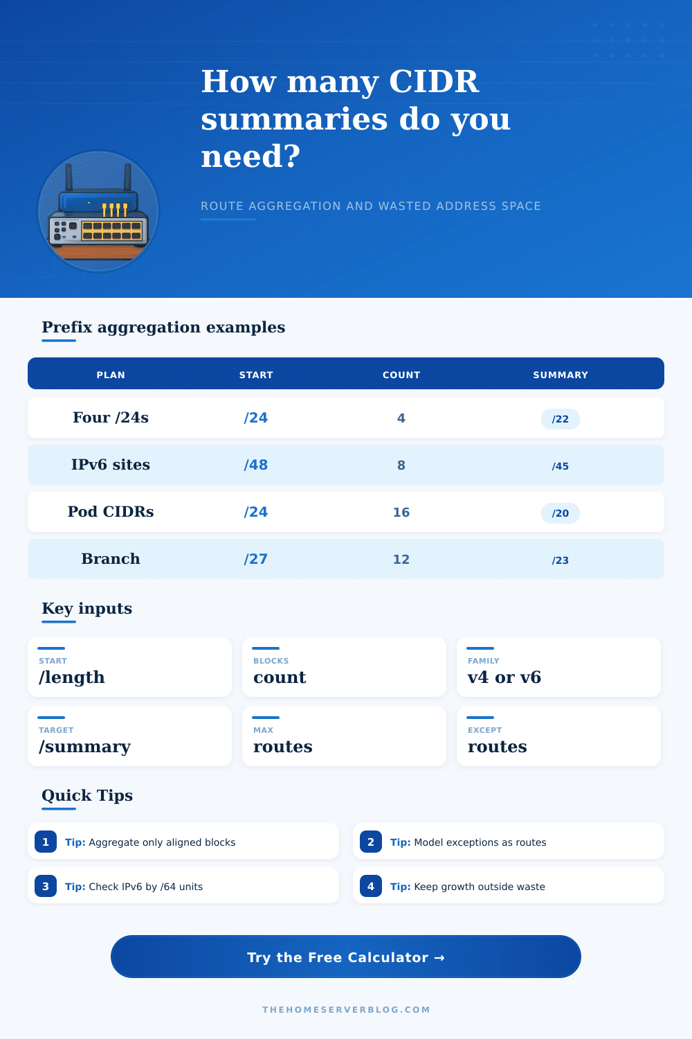
The page includes reference tables laying out familiar use cases: aggregating Kubernetes pod CIDRs; summarizing a bunch of /48s from an ISP into a single /45. Concrete examples bridge abstract binary math to practical infrastructure design. Remember that aggregates not only limit what is possible, but they are also part of your planning strategy. How aggressively do you want to pack today versus how much room should you reserve for future growth?
Don’t accidentally make it harder to scale up by summarizing too much. Keep growth free by leaving it in unused addresses. That’s where network design comes in: breaking the rules is the art. Sticking to perfection (in this case perfect alignment), can result in slower deployment. In some cases, advertising an additional route makes sense. In others, delaying a project until you’ve renumbered addresses does not make sense. With the calculator, you can measure that choice.
A vague worry about “wasted space,” or “too many routes” becomes something you can express as numbers and defend during your architecture review. You learn how to balance striving for simplicity against messiness and complexity of the real world. In summary: Prefix aggregation is a balance of flexible vs. Orderly. You want your routing table to be orderly so you can understand where things are going quickly, but you don’t want it falling apart when under pressure.
Knowing which boundaries have an exception and what that exception costs will help you build out networks that scale, while still being neat and tidy in your routing tables. The math doesn’t get different, but your view on the math does. Instead of seeing a long list of IPs, you begin to see address space as having a shape. From there you can make decisions more clearly and instead of fighting against the binary structure, you work with it. It’s this mindset switch that makes the difference between good network designs and great ones.