Splice Loss Calculator
Estimate link loss from fiber length, wavelength attenuation, fusion splices, mechanical splices, connector pairs, passive components, and required optical margin.
| Loss source | Count or length | Unit loss | Total dB | Planning note |
|---|
10GBASE-SR + OM3/OM4
Short 850 nm links with high fiber attenuation but limited distance. Best inside racks, rows, and small rooms.
10GBASE-LR + OS2
1310 nm single-mode campus links. Connector quality and splice count often matter more than cable loss.
10GBASE-ER + OS2
1550 nm extended reach optics with more budget. Watch receiver overload on short clean spans.
PON + Splitters
GPON and XGS-PON budgets are dominated by splitter loss, with splices and connectors consuming reserve.
| Component or fiber | Typical value | Conservative value | Where it applies | Field note |
|---|---|---|---|---|
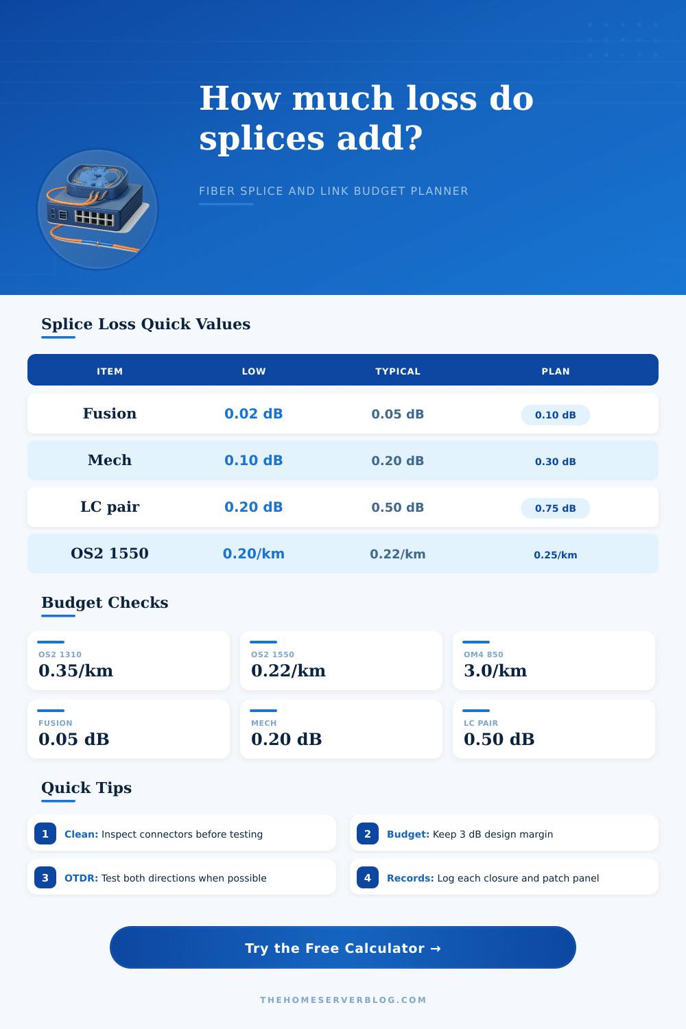
| Fusion splice | 0.02 to 0.05 dB | 0.10 dB | Permanent pigtail or cable joint | Use OTDR average, not only splicer estimate. |
| Mechanical splice | 0.10 to 0.20 dB | 0.30 dB | Emergency restoration or temporary repair | Plan higher loss and revisit later. |
| LC/SC mated connector | 0.20 to 0.50 dB | 0.75 dB | Patch panel, SFP, adapter sleeve | Dirty end faces can exceed the budget quickly. |
| OS2 at 1310 nm | 0.35 dB/km | 0.40 dB/km | 10G LR, 100G DR, many BiDi links | Common design value for single-mode. |
| OS2 at 1550 nm | 0.22 dB/km | 0.25 dB/km | ER, ZR, CWDM, long metro spans | Lower attenuation, but bend loss can rise. |
| OM4 at 850 nm | 3.0 dB/km | 3.5 dB/km | SR optics and short data center trunks | Distance limits are often bandwidth-limited too. |
You’re holding a light meter in your hand, looking at a flickering server while standing in a cold data center aisle. According to the schematic, this should work. The link map shows two kilometers. Your gut is telling you there’s something wrong. Optical budgets has an unfortunate tendency to die in the gap between theory and reality, typically due to growing drag from each tiny imperfection along the way.
On paper fiber optics are clean. In the field, loss accumulate one invisible scratch at a time.
How to Use the Optical Budget Calculator
Once you enter the number of events and fiber length, the calculator above do the rest, saving you from having to guess at exactly how many decibels each will consume. The tool divides the total attenuation into five categories: passive components, connector pairs, mechanical splices, fusion splices, and cable distance. Why? Because not all attenuation are alike.
Some loss is predictable physics. Cable attenuation is a known amount that increases steadily with distance based off type of fiber and wavelength.
Other loss involve humans. Splices and connectors depend on how well the technician aligned them and how cleanly they were made. They also depend on how skilled the technician was. A well-executed fusion splice should only be about 0.05 dB down. It’s reasonably robust; do it wrong and it can fails outright. But after forty on some long metro span, that starts adding up.
With this tool, you can number each one and see how much they add up to collective. Mechanical splices are a different animal, where you’re using index-matching gel or physical alignment sleeves, which tend to be more lossy on average (like 0.20 dB) and which will get worse over time as the gel dries out or the sleeves shift. Maybe use those in an emergency? But then it eats into your design margin quick.
The budget fails at connectors. While we all know that dirty connectors are a problem, I think folks don’t appreciate just how many dBs you add with each bad mating event. A seemingly good-looking LC pair could have tiny gaps or worn end-faces and still add 0.5 dB of loss. You can specify connector loss per pair on the calculator so you can model what happens out in the field vs. It is an ideal lab performance.
It also has a field for passive components such as muxes or splitters. Those are big hitters when you’re talking about a PON network where the splitter loss dominate the whole equation.
Margin is what makes or breaks a deployment. Receiver sensitivity plus transmitter power is a hard limit on optical budget. You can’t do much about it. Splices, connectors, cable loss and component drag are easy to calculate. What’s left over in dB is your safety net. When that goes to zero, the link may work today but probably won’t tomorrow after a bump to a patch cord or just settling in with some dust. A good rule of thumb from industry standards is to leave yourself at least 3 dB of reserve for both unforeseen and aging issues. This tool tells you if you make or break that mark by giving you a simple green light or red light before you cut a single piece of cable.
We are tempted to think of fiber as a copper wire; if the wires connect the signal flows. But that isn’t how light behaves. It reflects, it scatters, it bends at each interface. A speck of dust on an end-face can scatter just enough light to take the signal down into the noise floor of the receiver. And that’s why inspection is important, much more so than most people know. Math doesn’t clean a dirty connector, you have to clean it with your hands. The calculator tells you what is theoretically possible… Your hands tell you what you really got.
Do the math twice when laying out more complex links, particularly if they span several buildings or have any legacy gear. Assume greater losses with older connector types and be conservative with attenuation. Find out early in the design phase if you require an optical amplifier; don’t find out post-installation that your link is flaky. Their example tables on the page give typical parameter values for different fiber varieties and parts, so you can check your assumptions. You’ll see why 850 nm is good enough for intra-rack connections between switches and why single-mode reaches further at 1550 nm.
In short, math is realy more of a risk management equation than an arithmetic one. It makes you think about all of those physical interactions with light. You model them out individually so you can start to see what parts of the system are consuming your budget. Is it the large span? Too many patch panels? Is it someone’s dirty boots in the equipment closet?
Once you know where your loss lives, you can fix it before it becomes a ticket. Happy networks equal clean fiber, and the math will tell you precisely when you’ve crossed that line.