HomeServerBlog queue latency tool
Utilization vs Response Time Calculator
Estimate how queue wait and response time climb as a worker pool, database queue, VM, disk, Redis instance, or CI runner pool gets closer to saturation.
Queueing breakdown
Total expected time in system: queue wait plus service time.
Expected waiting time before a request reaches an available server.
Arrival load divided by total service capacity after burst multiplier.
Inbound request rate, adjusted by burst multiplier for peak planning.
Per-server completions per second, inverse of average service time.
Parallel workers, connections, cores, consumers, runners, or I/O lanes.
Erlang C estimate of the chance a request joins the queue.
Expected number of requests waiting in the queue during steady load.
M/M/1
Single server with exponential arrivals and service. It shows the classic latency explosion near 100% use.
R = 1 / (mu - lambda)M/M/c
Multiple equal servers with one shared queue. This calculator uses Erlang C for the main estimate.
Wq = C / (c mu - lambda)M/D/c approx
Low service variance reduces queue wait. Use deterministic mode for caches, Redis, and tight CPU loops.
about 50% WqPriority or batch
Priority and batch queues can help important work while increasing average or tail wait for other work.
factor adjusted| Queue discipline | Wait factor | Best fit | Practical note |
|---|---|---|---|
| FIFO / fair request queue | 1.00x | APIs, web threads, DB pools | Good baseline when work is similar and fairly scheduled. |
| Priority queue / noisy neighbors | 1.25x | Mixed importance jobs | Average wait rises when lower priority work is repeatedly displaced. |
| LIFO / newest first pressure | 1.15x | Interactive stacks under retry pressure | Can make old requests stale while fresh requests appear faster. |
| Batch drain / consumer poll | 1.35x | Consumers, CI, ETL | Polling and batch windows add waiting beyond pure service contention. |
| Low variance deterministic service | 0.55x | Redis, cache hits, fixed CPU work | Predictable service cuts queue wait compared with exponential service. |
| Utilization band | Expected behavior | Response time shape | Action |
|---|---|---|---|
| Under 50% | Comfortable headroom | Service time dominates | Measure p95 and keep watching bursts. |
| 50% to 70% | Healthy production range | Queue wait appears but remains controlled | Good zone for most home lab and small production pools. |
| 70% to 85% | Latency starts bending upward | Small traffic changes create visible wait | Add workers, lower service time, or shed burst traffic. |
| 85% to 95% | Near saturation | Response time becomes unstable | Treat as urgent unless the queue is intentionally batch oriented. |
| 95% and higher | Saturation cliff | Wait time can grow without bound | Reduce arrivals or increase capacity before retries pile up. |
| Scenario | Typical service time | Typical target | Watch metric |
|---|---|---|---|
| API Worker Pool | 10 to 80 ms | 100 to 250 ms | p95 response, worker busy percent, queue length. |
| Database Connection Queue | 5 to 60 ms | 50 to 150 ms | pool wait, active connections, lock wait. |
| CPU Saturated VM | 20 to 200 ms | 150 to 500 ms | run queue, CPU steal, load average per core. |
| Disk I/O Queue | 2 to 30 ms | 20 to 100 ms | await, queue depth, IOPS saturation. |
| CI Runner Queue | 60,000 ms and up | minutes | queued jobs, runner busy time, retry count. |
| Capacity lever | Formula effect | When it helps | Tradeoff |
|---|---|---|---|
| Add servers | Raises c x mu | Parallel work with a shared queue | Can hit locks, partitions, or connection limits. |
| Improve service time | Raises mu | Slow handlers, queries, builds, or I/O paths | Requires profiling and code or storage changes. |
| Smooth bursts | Lowers effective lambda | Retry storms, load tests, cron spikes | Needs backpressure, jitter, or rate limits. |
| Increase safety buffer | Lowers safe arrival rate | Unpredictable workloads and shared hosts | More idle capacity by design. |
| Split queues | Changes arrival mix | Priority lanes or noisy tenants | Can starve low priority work if unmanaged. |
Until it is not. Until use gets high enough. You can keep running your server pool at half capacity for weeks and have no problem. Then you get it up to around eighty percent and suddenly things starts getting sluggish. But they don’t just kind of inch along, they go from good to bad in milliseconds.
It makes sense in retrospect. At the time, it look like something has gone wrong with your code or your servers is unstable. Usually it’s not. You’re closer to full load than you think. Every millisecond of service is now becoming minutes spent waiting by customer.
Why Your System Slows Down at High Use
To make those calculations, the calculator splits out queue wait versus active processing. And this split is important: It’s the thing that most people are trying to tune when they should of tuning something else entirely. Latency goes up? The team adds some database indexes or optimizes their code. They don’t realize that there’s a chance it could just be sitting in a queue waiting for its turn on the CPU.
Queue wait can grow much larger then your baseline. This can happen even if you have a fixed service time of twenty milliseconds and utilization reach ninety percent. The tool estimates this delta, so you can get an idea of how far you’re stretching things and how close you are to slowing things down.
To understand arrival rates, you have to look beyond average. Real traffic isn’t smooth… It come in bursts. Your load test might show that your pool handles two hundred requests per second just fine. But in production, nothing ever shows up in a nice stream. It shows up as spikes. Suddenly, twice as many users show up; or one of your downstream service has a retry storm. That triples your arrival rate… for thirty seconds. If your baseline use was already at seventy percent, that spike pushes you straight into a critical state.
That’s why the calculator lets you define a burst multiplier with exact precision. It makes you model chaos. Not just calm.
The duration of a queue depends on queue discipline too. Fair (first-in first-out) queues serves each request in turn; they’re fair, but every request is treated the same. Priority queues allows workloads that must run quickly to jump the queue, while often making everyone else’s wait time worse. Batch processing introduces additional delay: Consumers poll for work instead of responding immediately. These structural decisions change the mathematical equation.
An erratic workload perform poorly under load, while a deterministic workload with low variance always does well. Why? Because the scheduler know what to expect from the next task. The page lays out these considerations in a reference table, so you know which to tune your expectations around.
The majority of us get this wrong. We size for the mean. Because we do, our systems remains exposed to outlier events. That 20% safety buffer, which is not simply wasted hardware, protects from variability. It cushions the system from unexpected user actions, unevenly distributed CPU core usage, and network latency jitter.
Any small hiccup pushes use above the threshold. When utilization exceeds capacity, you gain little benefit from increasing server count. You are better served dropping non-urgent tasks or slowing down non-time sensitive requests than adding yet another machine to your saturated queue.
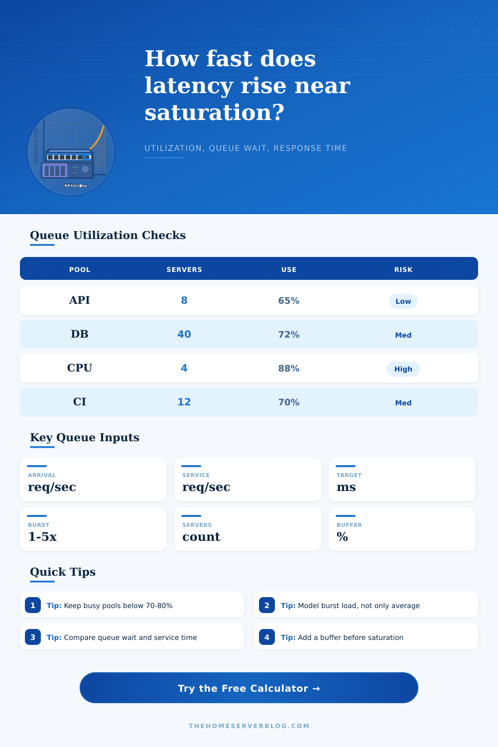
We don’t want our use to be zero, either. That’s wasteful. Typically, your sweet spot is somewhere around fiftyish to seventyish percent use. Above that threshold, you have some headroom so you can handle bursts without blowing out resources, but below that threshold you’re reasonably cost-efficient. Beyond eighty five or ninety percent, you start getting into the zone of diminishing returns, which is very nonlinear: you get exponentially more wait time for linearly more load.
That may seem small, but it makes a big difference. It’s much cheaper to monitor that usage number than debug a timeout incident at 3am. Get an alert from the tool when you are getting into trouble. Do not wait until customers complain about long queues.
The bottom line: Response time is ultimately a balance of chaos and capacity. It’s impossible to predict what people will do with a product, but it IS possible to predict how much slack you need in your system. If you model for bursty behavior, and honor the safety buffer, you’ll be able to make unanticipated latency a variable factor, rather than an impossible obstacle.
Don’t let this math catch you off guard, it gets very unforgiving when approaching saturation.