Ceph Erasure Coding Calculator
Estimate Ceph EC k/m pool efficiency, raw and usable capacity, PG count hint, failure-domain fit, object padding, and recovery read amplification.
| EC profile | Width k+m | Raw overhead | Failure tolerance | Typical home lab use |
|---|---|---|---|---|
| 2+1 | 3 OSDs minimum | 1.50x raw | 1 shard | Small test pool, not much spread |
| 3+2 | 5 OSDs minimum | 1.67x raw | 2 shards | Compact cluster with extra parity |
| 4+2 | 6 OSDs minimum | 1.50x raw | 2 shards | General NAS data and backups |
| 6+2 | 8 OSDs minimum | 1.33x raw | 2 shards | Balanced media and VM images |
| 6+3 | 9 OSDs minimum | 1.50x raw | 3 shards | Archive pool with more fault room |
| 8+3 | 11 OSDs minimum | 1.38x raw | 3 shards | Large rack-aware object pool |
| 10+4 | 14 OSDs minimum | 1.40x raw | 4 shards | Cold object data on wide clusters |
| PG planning item | Formula used here | Why it matters | Practical note |
|---|---|---|---|
| Base PGs | OSDs x target x share / width | EC PGs touch k+m OSDs | Round to a power of 2 |
| Acting set width | k + m | Each PG maps that many shards | Needs enough distinct OSDs |
| Autoscaler check | Use final cluster stats | Balances pools by bytes | Prefer Ceph mgr advice |
| Too few PGs | Hot OSD risk | Less placement spread | Watch OSD fullness skew |
| Too many PGs | Memory and peering load | More metadata work | Increase carefully |
| Object size | 4+2 stored | 8+3 stored | Padding sensitivity | Best fit |
|---|---|---|---|---|
| 64 KiB | 6 stripe units | 11 stripe units | High | Prefer replicated metadata |
| 1 MiB | About 1.5 MiB | About 1.4 MiB | Medium | Small object buckets |
| 4 MiB | About 6 MiB | About 5.5 MiB | Low | RBD or object data |
| 16 MiB | About 24 MiB | About 22 MiB | Low | Bulk media and archive |
| Failure domain | Input meaning | Minimum useful count | Risk if short | Planning action |
|---|---|---|---|---|
| OSD | Each shard on a disk | k+m OSDs | Host loss may lose many shards | Use only in tiny labs |
| Host | Each shard on a node | k+m hosts | Undersized acting sets | Add nodes or lower width |
| Chassis | Each shard per chassis | k+m chassis | Chassis fault can exceed m | Use device classes too |
| Rack | Each shard per rack | k+m racks | Placement may be impossible | Use smaller k/m profile |
| Room | Each shard per room | k+m rooms | Stretch design pressure | Confirm CRUSH map first |
The math said you needed a certain amount of raw storage across your hard drives to store your media library and virtual machines securely. You purchased those drives. Then you configured an erasure coding pool and saw that your usable capacity was significantly below what you expected. If this sounds familiar, then you’ve transitioned from a basic replication pool to a Ceph erasure coding pool and are wondering how this could be.
It’s not. It’s simply arithmetic; an exchange between faster recovery time and more efficient usage. Before you initialize your very first disk, understand that tradeoff so that you don’t build out a cluster which might look great on paper, but doesn’t perform well in reality.
Why Your Storage Space is Smaller Than Expected
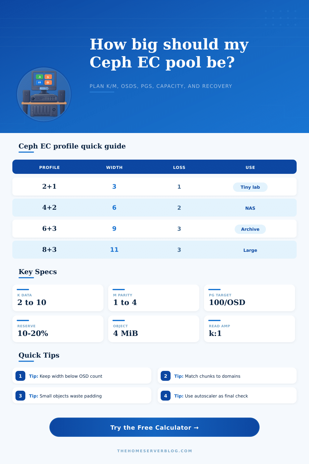
Plugging in your data and desired level of parity turns over the work to the calculator, which will do the math for you. The calculator handles the math once you plug in your data and parity requirements, which removes the guesswork from coefficients and conversions. With a 4+2 profile, it’s telling you that your storage efficiency is about sixty-seven percent; four parts are actualy data, while two are parity.
Sounds good until you realize this means if you lose a single shard, the system has to read all four others and try to put together what was lost. The larger your stripe, the more network traffic you’re going to create as things rebuild themself. It is small stuff but it is important when you want to get your data back fast without clogging up your network bandwidth.
Where most home lab admins go wrong is choosing the correct failure domain. Whatever CRUSH map you create, it should spreads its shards over hosts, so make sure you have enough physical machine to match that setting. For a profile of 4+2, for instance, you’ll need at least six different hosts (which means one shard per host). Anything less (such as four hosts) and your pool’s placement rules will conflict and your pool won’t be healthy.
It doesn’t matter how much you fiddle with software; you can’t fake geography. Your hardware has to back up whatever geographic distribution strategy you choose in your settings. You should also consider object size, which isn’t shown in capacity charts. With erasure coding, the idea is to split data into stripes, and smaller objects may be padded out so they take up full stripe. For example, if a wide EC pool has stripes that require padding, a little text file will occupy as much on-disk space as big video file, since it’s padded out to the next stripe boundary. That’s one reason why erasure coding tends to make more sense for bulk storage, as opposed to a workload involving many small but metadata-rich objects. Replication may actualy result in fewer wasted bytes (and higher performance) compared to erasure coding if your workload consists of millions of small files.
The other thing that takes some forethought is how you plan out your placement groups. If you have too few, you’ll end up with hot spots when some drives fill up before others because they’re unevenly distributed among OSDs. Having too many PGs makes cluster peering tasks slower and also increases amount of memory the monitors use. Again, there’s a hint provided by the tool based off your target load and number of OSDs but you should confirm it against the Ceph autoscaler after the cluster is live. It doesn’t give you the final decision; it gives you a place from which to tune.
The price of efficiency you don’t see is that your recovery gets amplified. If a drive dies on a pool where there are replicas, it just copies data from another drive. With an EC pool, it has to pull out chunks from several survivors and stitch them together to recreate the parity. So with a 10+4 profile, saving a lot of disk space versus replicating, if a shard dies, then you have to read in ten others to rebuild it. It causes a lot of I/O on those other drives while you’re trying to recover. You pay less operationally when things are fine; you just get more capacity, but you would of paid more operatively when something goes down.
Your goal isn’t perfection, it’s matching your storage approach to your true tolerance for complexity and risk. Wider profiles work if you’ve got lots of drives and want maximum durability. Simpler ones will help you stay in control if your CPUs is weak or your network bandwidth is limited. Once a pool exists, changing its profile is hard; that’s why getting the starting layout correct helps ensure lasting growth (not a maintenance headache) as your cluster scales. Go with what makes sense to you, check the capacity implications, and use the numbers to inform your hardware buying decisions, not guesswork.