Average Load Calculator
Interpret Linux 1, 5, and 15 minute load averages against CPU cores, runnable tasks, I/O wait, steal time, background jobs, and reserved headroom.
nproc or lscpu.top load task state or vmstat r.top wa, iostat, or node exporter.1 minute
Best for catching a bursty compile, media scan, Docker pull, backup start, or unexpected queue spike.
5 minute
Best for deciding whether the machine is recovering or slowly building a sustained backlog.
15 minute
Best for capacity planning because short spikes are smoothed and persistent demand is visible.
Runnable queue
Best cross-check for CPU pressure because load also counts tasks waiting on uninterruptible I/O.
| Adjusted load per core | Server condition | What it usually means | Home lab action |
|---|---|---|---|
| 0.00 to 0.50 | Comfortable | Interactive work and services have ample CPU time. | Keep normal monitoring and avoid over-tuning. |
| 0.50 to 0.70 | Healthy busy | Docker, NAS, or VM work is active but not queueing heavily. | Good target for mixed always-on servers. |
| 0.70 to 1.00 | Near full | CPU can keep up, but headroom for spikes is shrinking. | Check noisy jobs, cron timing, and service limits. |
| 1.00 to 1.50 | Queued | Average demand is above available CPU capacity. | Reduce work, move jobs, or add CPU capacity. |
| 1.50 and above | Saturated | Tasks are waiting long enough to affect latency. | Investigate immediately with top, iostat, and ps. |
| Signal | Linux field | Concerning range | Likely bottleneck |
|---|---|---|---|
| Runnable tasks | vmstat r | Above core count | CPU queue, thread burst, or too many workers |
| I/O wait | top wa | 8% to 15%+ | Disk, ZFS scrub, swap, NFS, or slow USB storage |
| CPU steal | top st | 3% to 10%+ | VPS host contention or oversubscribed hypervisor |
| Blocked tasks | vmstat b | Repeated nonzero | Uninterruptible I/O, storage latency, or driver wait |
| Run queue trend | uptime | 1m above 15m | New spike; verify if it decays after the job ends |
| Workload profile | Recommended target | Watch first | Useful command |
|---|---|---|---|
| Home Assistant host | 0.45 to 0.60/core | Latency and database writes | top -o %CPU |
| NAS with ZFS | 0.55 to 0.75/core | I/O wait and ARC pressure | iostat -xz 1 |
| Plex or Jellyfin | 0.70 to 0.95/core | Transcode workers | ps -eo pid,comm,pcpu |
| Proxmox node | 0.60 to 0.80/core | Steal, VM ready time, backups | htop |
| CI runner | 0.85 to 1.10/core | Batch queue depth | pidstat 1 |
| Named scenario | Typical cores | Normal load band | Common cause of high load |
|---|---|---|---|
| Raspberry Pi 4 Home NAS | 4 | 0.4 to 2.2 | USB disk wait, Samba copies, media indexing |
| Intel N100 Docker Host | 4 | 0.8 to 3.0 | Container restarts, backups, log processing |
| Proxmox Mini PC Node | 8 | 1.2 to 5.5 | VM backup compression and oversubscription |
| TrueNAS ZFS Scrub | 8 | 2.0 to 6.5 | Disk wait during scrub or resilver |
| VPS Noisy Neighbor Check | 2 to 4 | 0.3 to 2.0 | CPU steal from the virtualization host |
wa is high, check disks, swap, network storage, ZFS scrub activity, and blocked tasks before buying more CPU.Check the numbers. Run a quick command from memory. Two point five for a four core machine sounds fine. But then you remember your backups is sitting stuck in an uninterruptable sleep state. The trap with Linux load averages is that they look simple on the surface, but you might see numbers that seem fine until you realize whole system feels sluggish.
They’re simple metrics that looks simple on the surface. However, they hide a complex story of virtualization overhead, CPU pressure, and disk I/O. Most people see a number and assume it means processor usage. In fact it’s measuring the number of runnable processes plus those waiting for resources. That makes a difference when you’re trying to decide whether to tune your server better or add some hardware.
Understanding Linux Load Averages
That’s where the calculator above comes in. It helps untie that mess by allowing you to put your actual load into a set of comparisons with various limits. Rather than viewing a number in isolation, it factors in core count, I/O wait, etc. It shows you if a bunch of background jobs is skewing things. It allows you to enter average values over one minute, five minutes, and fifteen minutes, so you can see the trend. It then changes the math to match your workload profile.
A Plex transcode box has different requirements than a database server. The former want burstable power for brief periods; the latter wants constant availability. This helps avoid over-reacting to a temporary spike and ignoring a slow burn that will take down your services later.
These are time based snapshots of load averages. The one minute average is going to be very jittery, because it will pick up instantaneous spikes like when a media scan kicks off. That’s why the fifteen minute average is what you want to look at for capacity planning; it smooths over the noise and reveals sustained load. When the fifteen minute load remain higher than your core count, you’re really running hot. Tasks get queued and wait, users perceive sluggishness, and backups start failing. The five minute average is somewhere in between; it’ll help you decide whether a spike is improving or getting worse. Knowing which window is relevant for your decision will keep you from panicking with harmless fluctuations.
Most of your diagnostics are going to fail on I/O wait. Your CPU isn’t busy? Your load average is high? Disk issues are far more likely to cause a high load average than CPU starvation. Even if your hard drives can’t keep up with read requests and other processes end up blocking on storage operations, those processes still get counted towards the load. Therefore, it’s worth looking at I/O wait percentages and blocked tasks when you observe high load with low CPU utilization (look at top). Swapping out to disk and reading from slow USB drives will quickly jack up the numbers here. Typically, solving storage bottlenecks will reduce the load average more effective than throwing an additional processor core at it.
The other issue is stolen time (which isn’t reflected in usage statistics). Your virtualized environment’s guest OS can give away CPU cycles to host operating system and other tenants on VPSes or cloud instances. Steal time eats into your available capacity by reducing your effective resources. If you’re seeing high steal numbers and occasional slowness, you might want to contact your provider. They could be overselling their hardware. There’s no way to optimize this locally. You’ll either have to switch to dedicated resources or upgrade your plan if performance still suffers under heavy load at certain times.
Background jobs are another thing that affects your perceived performance. A scheduled task rotating logs, updating packages, or scrubbing a database may cause some spikes in your load metrics. So if you see something spike for a minute but know there’s a big job running, don’t freak out, let it complete then look at the longer term (the 15 minute trend). Run those big jobs during off-peak times and you’ll be fine in terms of daytime usability.
Limit resources for less critical processes; don’t let them starve interactive services. You want sustainable headroom, not maximum use. Running a healthy amount below the core count allows for any kind of surge. For mixed workloads, you might find that ~70% per core is a good sweet spot. This provides a buffer for those background tasks while minimizing impact on user-facing apps. Even if your server is doing something (i.e., actual work), you still want it to feel responsive.
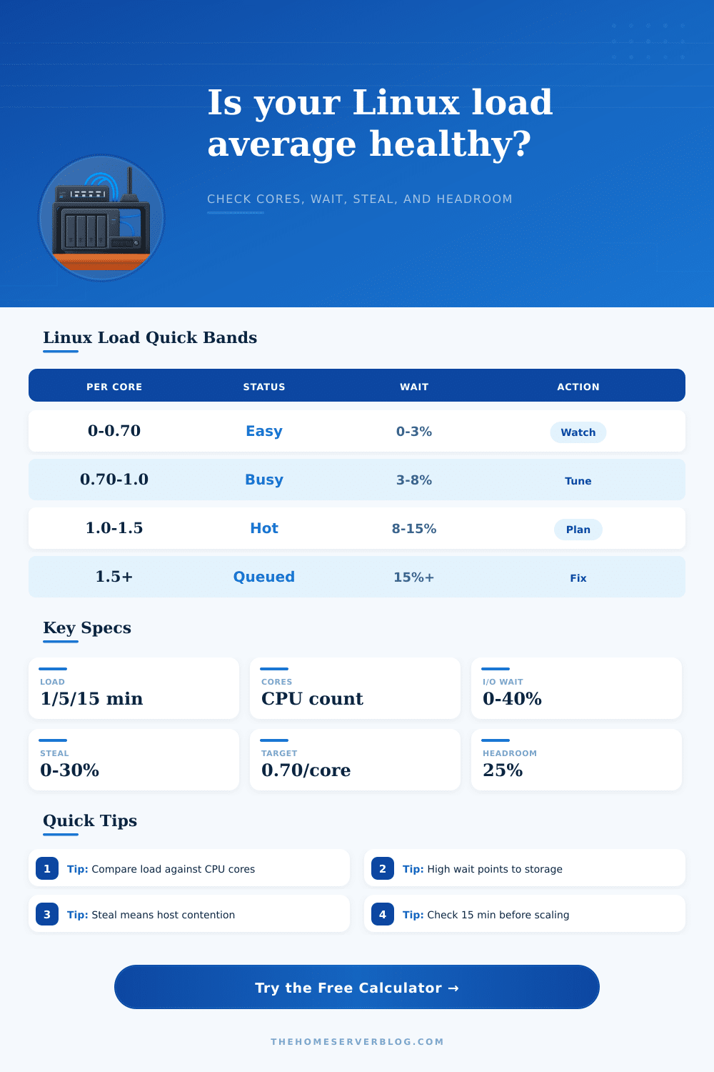
This is nicely explained in the reference table on the page, which maps server conditions to an adjusted load band. Abstract numbers turn into actionable status reports. It’s all about tracking behavior
In conclusion, tracking isn’t about getting to 100%. It is learning how your particular configuration responds when stressed normally. You learn what causes the spikes and why, and you change your own expectations to match. If the system holds up just fine with a bit more load during certain periods of obvious maintenance, that’s fine!
That’s where most of the magic lies: knowing what the hell is actualy being reported by those three easy-to-digest numbers. When you know the distinction between “waiting” resources and “processing” power, those numbers stop feeling like they’re being randomly selected from a hat. Instead, they feel like a legitimate dashboard of your digital home. Track the trends, respect the headroom, and use the data to inform the next step, not fear.