Database cache planning
Buffer Pool Hit Ratio Calculator
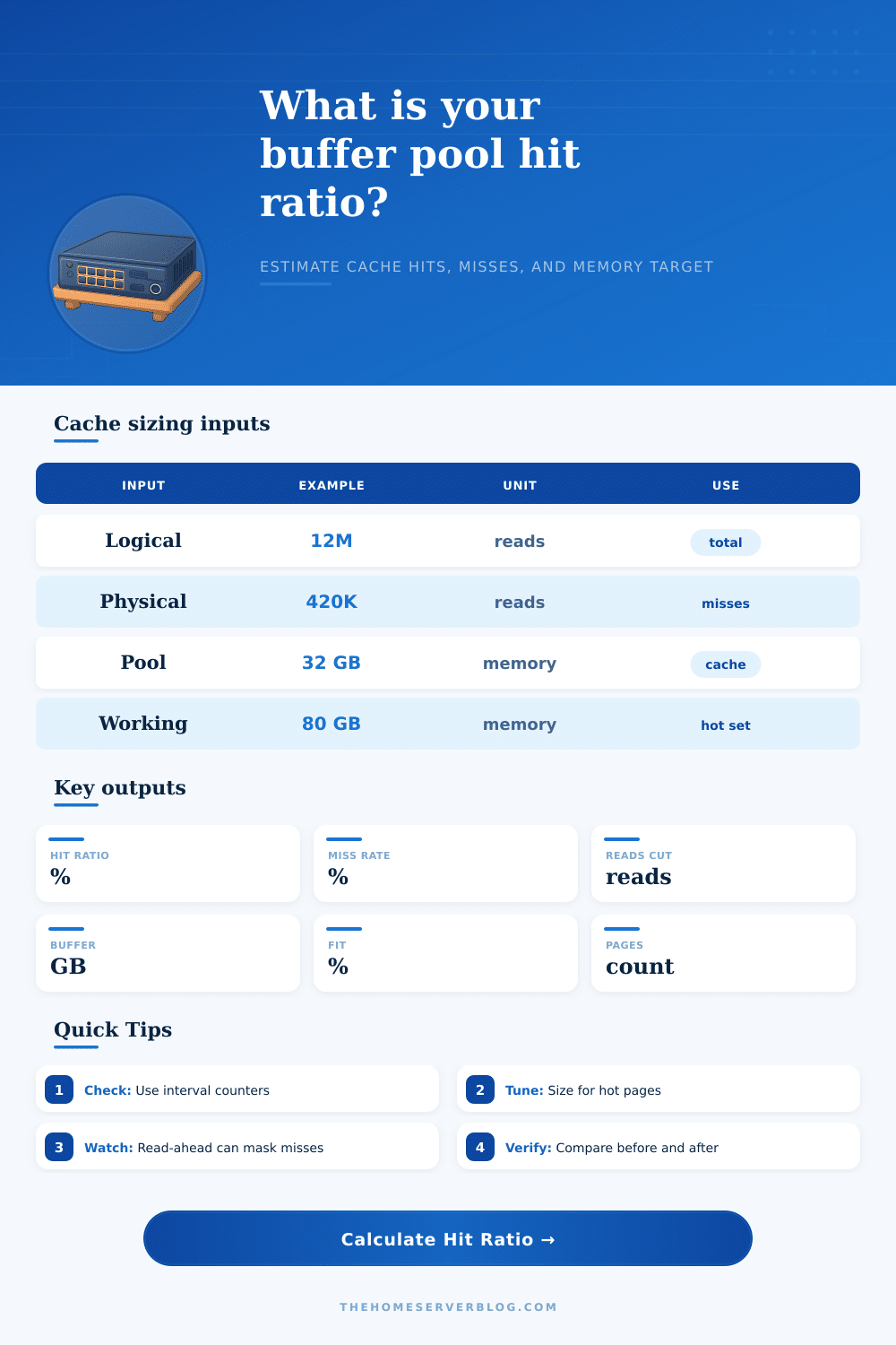
Estimate cache hit ratio, miss rate, avoidable physical reads, and a practical buffer pool target from logical reads, physical reads, current memory, working set size, page size, read-ahead, dirty pages, and target hit ratio.
Logical reads
All page requests made by queries or the storage engine, including reads satisfied from memory.
12.0MPhysical reads
Page requests that missed cache and required storage, prefetch, or filesystem reads.
420KWorking set fit
How much of the hot data can fit in the current pool after dirty page pressure.
33%Clean cache
Estimated buffer space left for reusable clean pages after dirty page share is removed.
28.2 GB| Database engine | Main cache metric | Typical healthy range | Counter caution |
|---|---|---|---|
| MySQL InnoDB | Buffer pool hit ratio from logical versus disk reads | 99%+ for stable OLTP, lower during scans or warmup | Check over an interval; cumulative uptime counters hide recent changes. |
| SQL Server | Buffer cache hit ratio plus page life expectancy and read latency | High 90s is common, but PLE and waits matter more alone | Very high hit ratio can still coexist with memory pressure or bad plans. |
| PostgreSQL | Heap and index hit ratios plus OS page cache behavior | 95% to 99%+ depending on workload and scan volume | shared_buffers is only part of the cache because Linux page cache is important. |
| Oracle | Buffer cache hit ratio and physical read waits | Usually high for OLTP, but wait events guide action | A single ratio should not override DB time, waits, and segment-level reads. |
| MongoDB WiredTiger | Cache bytes, pages read into cache, eviction pressure | Depends on document working set and filesystem cache | WiredTiger cache and OS cache work together, so memory must be split. |
| Redis with persistence | OS page cache and latency spikes around persistence or swap | Application hit ratio is separate from disk persistence behavior | A Redis key hit ratio is not the same as storage buffer cache performance. |
| Observed hit ratio | Typical meaning | Best next check | Possible action |
|---|---|---|---|
| 99.5% to 99.99% | Excellent cache reuse for most OLTP systems | Confirm latency, lock waits, and write stalls | Do not add memory unless misses are expensive or bursty. |
| 98% to 99.5% | Often acceptable for mixed workloads or fresh cache | Look at physical reads per minute and slow query plans | Add targeted indexes or modest cache if random reads dominate. |
| 95% to 98% | Potential pressure for latency-sensitive applications | Separate random misses from read-ahead and table scans | Increase useful cache, tune queries, or partition hot data. |
| 90% to 95% | Likely cache misses, scan-heavy reporting, or undersized memory | Check top physical-read objects and storage latency | Reduce working set, add memory, or isolate analytics. |
| Below 90% | Usually unhealthy for random OLTP, unless workload is intentional scanning | Validate counters, warmup state, and backup or ETL activity | Fix query shape before relying only on a larger buffer pool. |
Memory-first tuning
Best when misses are random, repeated, and storage latency is high. Increasing cache helps only if the extra memory holds pages that will be reused.
Query-first tuning
Best when a few queries create most physical reads. Better indexes, narrower scans, and partition pruning can cut misses without adding RAM.
Workload isolation
Best when reporting or ETL flushes a healthy OLTP cache. Replicas, read pools, or scheduled windows protect the hot transactional set.
| Workload | Working-set target | Read-ahead signal | Dirty-page concern |
|---|---|---|---|
| Random OLTP | Fit hot indexes and hottest table pages first | Low read-ahead share is expected | Keep flush pressure stable so clean pages remain reusable. |
| Read mostly API | High fit ratio can produce very low physical reads | Moderate prefetch during range lookups is fine | Dirty share is usually low unless background jobs write heavily. |
| Mixed reporting | Fit OLTP hot set, not every reporting scan | High read-ahead means scans are influencing the ratio | Large temp writes or batch updates can crowd the cache. |
| Warehouse scans | Buffer pool may not need to hold full fact tables | High read-ahead is normal and not always bad | Batch loads and checkpoints should be planned around write bandwidth. |
| Time series | Fit recent partitions, active indexes, and metadata | Older range reads may show scan behavior | Ingest bursts can raise dirty pages quickly. |
Even if the logic is same, you discover that one query that used to complete in thirty milliseconds now take three seconds. Checking the indexes and looking at execution plan reveals nothing. You think maybe problem is network, but oftentimes the culprit is lurking in memory. The data you require were evicted from buffer pool. Another piece of data wanted that spot more desperateley. It feel like a physical limit on how fast your app can run.
Once you enter logical and physical read counts into calculator (above), it’ll crunch numbers for you. But you still need to understand what they mean. A logical read happen whenever your database engine request a page of data. And a physical read is only when that request was made but couldn’t find the page in RAM so it had to go get it off disk. The difference between these two show how much work your storage layer are doing. This impacts consistency and throughput.
Understanding Database Memory Issues
A high hit ratio is viewed as some sort of badge of health by most folks, and it all depends on context. An engine with a ninety-nine percent hit ratio may be awesome for handling a random lookup OLTP workload. That’s great; every millisecond spent waiting for disk is precious. The same ratio can be confusing on data warehouse doing big sequential scans. In that case, the engine are deliberately grabbing data in bulk to feed the scan, which makes sense because the scan relies on that data.
The read-ahead activity is accounted for by ability to adjust the read-ahead setting on the calculator. Useful cache misses is distinguished from unavoidable cache misses due to big table scans. That come into play in determining whether to rewrite a query or invest in additional RAM.
The dirty page share is another quiet trap. As your app writes out data, that memory will contain dirty (modified) pages. That take up space in the buffer pool and it won’t be used for read requests until it gets flushed to disk. In other words, your effective cache size decrease a lot if your write load are significant. You still have all that memory allocated but less of it is available to you.
Perhaps you’re seeing a hit ratio drop off, so you conclude that you must add more memory. Maybe instead there’s a problem with flush latency or perhaps too-frequent checkpoints. Subtracting the dirty overhead from your cache size show how much clean memory is actualy available to you. This provides a more accurrate picture of the memory you can reuse.
Perhaps the single most important thing to tune correctly on this machine is working set size. How much memory does your application actualy use when under load? How many gigabytes of actual data does your app touch? If you’ve got a working set size of 12 gigabytes and allocated 32 gigs, then you’re wasting 20 gigs of memory. You’ve got 20 gigs of cold pages sitting there doing nothing.
In fact, adding more memory don’t help unless it contains more frequent used pages. When your cache exceeds your working set, adding more RAM will provide diminishing returns. You don’t have any new data to keep warm.
Under the hood, database engines such as SQL Server, PostgreSQL, and MySQL caches differently. But they also share the same basic tradeoff: what to store in memory versus what to pull from disk. The table on this page provide reference values for what is a generally healthy range of values. Use it to benchmark your system against industry standards. Keep in mind that benchmarks are static while workloads are dynamic. Always measure performance across a representative period of time. Do not look at total statistics gathered since the system started.
But in truth, I don’t think any of this is really about the magic number that makes it 99.9% instead of 99.8%. What you’re trying to do with a buffer pool is eliminate the costly physical reads. These are what give rise to latency spikes. You want to make sure the stuff you care about the most is in the buffer pool at the time you need it.
Run the calculator to get your starting point. Dig in on which objects is missed the most. In many cases a single bad join or missing index will skew your number more than any lack of memory would of. Tweak the shape of the workload, and numbers will generaly change as well.