Least Connection Distribution Calculator
Model how least-connections load balancing distributes fresh sessions across uneven backends, long-lived sockets, degraded nodes, surges, and maintenance drains.
| Algorithm | Selection signal | Where it behaves well | Watch carefully when |
|---|---|---|---|
| HAProxy leastconn | Fewest active connections among eligible servers | Long TCP sessions, RDP, MQTT, database gateways | Nodes differ in CPU speed or request cost |
| NGINX least_conn | Fewest active proxied connections | HTTP keep-alive, upstream pools, uneven request duration | One upstream has higher latency but same connection count |
| Envoy least_request | Low active request count, usually with random choices | High request volume service mesh traffic | Bursts arrive faster than metrics update |
| Weighted least connections | Connection count divided by server weight | Mixed hardware, larger nodes, GPU workers, partial capacity | Weights are copied from CPU count without real testing |
| Scenario | Typical active pattern | Lifetime driver | Least-connection concern |
|---|---|---|---|
| WebSocket chat | Hundreds to thousands per node | Users leave browser tabs open | New nodes start empty and receive a catch-up wave |
| Long polling API | Short waves that still overlap | Client polling timeout and retry cadence | Surge multiplier can briefly dominate the count |
| Database proxy pool | Stable but sticky connection pools | Application pool idle timeout | Drain time follows client pool recycle behavior |
| Media transcode farm | Few but heavy active jobs | Job duration rather than socket duration | Slow workers need a meaningful penalty |
| Metric | Good range | Investigate | Operational meaning |
|---|---|---|---|
| Projected balance spread | 0% to 15% | Above 25% | Some nodes are still carrying a materially larger share |
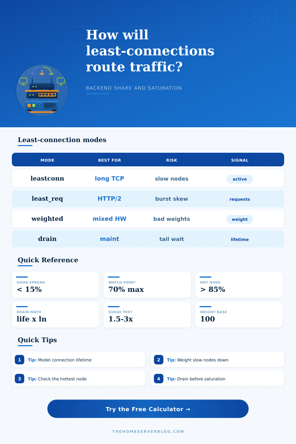
| Max-node saturation | Below 70% | Above 85% | The hottest backend is near its connection ceiling |
| Next-routing share | Near the expected least group size | One empty node gets most new sessions | Autoscale or maintenance changes may create catch-up pressure |
| Drain completion time | Matches maintenance window | Longer than deploy window | Existing sessions need shorter idle timeout or staged drain |
| Platform | Connection count source | Weight source | Drain signal to model |
|---|---|---|---|
| HAProxy | Server current sessions or scur | Server weight after health checks | MAINT, DRAIN, or zero effective weight |
| NGINX upstream | Active upstream connections from status module | Upstream server weight | Marked down or removed from upstream rotation |
| Envoy | Cluster upstream active requests | Endpoint locality and priority weighting | Health removal, outlier ejection, or zero load assignment |
| Database proxy | Backend pool active client sessions | Replica capacity or role-aware weight | Read-only pool removal before maintenance |
On paper, least connection routing seem straightforward. Send the next request to server with smallest number of open connections, and everybody lives happily ever after.
Reality is anything but static. Traffic patterns fluctuate. Server capacity vary. What starts out well-balanced using fewest connections can quickly become unbalanced. People assume that because system balances based off connections it also will balance based on load. That’s the source of most capacity surprises in production environments.
Why Least Connection Routing Is Not Perfect
Connections aren’t equal unit of work. One request uploading a large high resolution image take up one unit of capacity. An idle chat window over a websocket takes up another. If you think they’re interchangeable then you create hidden bottlenecks which will only manifest themselves when you are already swamped.
Once you know what to put where, that’s when the calculator above do the work. It spares you having to guess at how things will fill up during a surge. But more importantly it helps you understand why those numbers act like they do.
Look at the slow backend penalty setting. Half of your nodes might be older hardware, or maybe they’re doing something else heavy. Whatever the case, they can’t handles as many simultaneous tasks as well. The load balancer think the raw connection count on those nodes is low, so it treats them like empty seats. But really, they’re struggling inside.
A penalty adjust the system’s perception of those nodes and makes it think they’re busier than they actualy seem. So the fast ones aren’t sitting idle while the slower ones gets crushed. That makes all the difference between a naive algorithm and an intelligent one.
Another thing that surprises teams is lifetime of the connection. Short-lived HTTP requests burn through your pool and are dropped off rapidly, leaving the balancer free to route traffic to other nodes. Long-lasting websockets and other long lived connections such as database proxies hang around for hours or even minutes. What happens is there’s a kind of lag in the system. The routing decision you took ten minutes ago affects traffic today. A node may have been overloaded for just a few moments at the start of the day but will still be hot several hours later, purely because those session haven’t expired.
The tool models this decay and tells you how long it will take for an imbalanced pool to return towards balance. It can show that sometimes the recovery is slower then you expected, particularly if the average session duration has stretched out.
Take a look at the max-node percentage and you can see how close we are to saturation risk. It’s not just a warning light; hitting eighty-five percent of the backend limit means a timeout or dropped connections are coming. That’s marked on the reference table on the page as a critical watch point. As soon as one node gets close to that ceiling, new traffic has to be pushed over to the other servers. This raises their counts as well. It becomes a cascading failure until there is no room left for any more.
This is why the hottest node should of been monitored rather than average of the pool. Your average may look healthy but one server is dying. What you want to know is where the pressure is building up.
There are timing issues with draining nodes for maintenance too. The least connection algorithm does not force any existing sockets closed. It will just stop sending new traffic to a marked-out server. This means that how long the drain takes is completely dependent on when clients choose to hang up. Depending on whether your application pools retain idle connections or if your users leave their browser tab open, the node will remain in service well past the point where you pulled it out of rotation.
Understanding the decay here lets you plan for realistic maintenance windows. A simple flip of the switch isn’t enough. You need to wait until the session expires naturaly. This could take longer then your deployment slot can accommodate.
And the trick lies primarily in knowing what it is (and isn’t) measuring. Load is load; connection count is a proxy for load. When requests are evenly distributed by duration and cost, then it is fine. When they’re not? It’s like wearing a blindfold. You can adjust your penalties and weights to make up for it, and teach the algorithm the secret truth behind every single socket.
The point isn’t that every node should be exactly even at any specific moment, because it won’t. Thatd be impossible. The point is that it shouldn’t crash one node while another node coasts along. The point is to manage the flow such that the system doesn’t gasp but instead breathes. Ultimately, load balancing isn’t so much math as it is patience. Rules that admit to not being perfect are the way you smooth out the chaos.
The inputs are your understanding of user habits, the application behavior, and the hardware. Get those correct, and distribution just happens. Ignore them, and you’ll be running around following shadows on a dashboard full of red alerts.
Least connection routing is only as good as the context you give it.