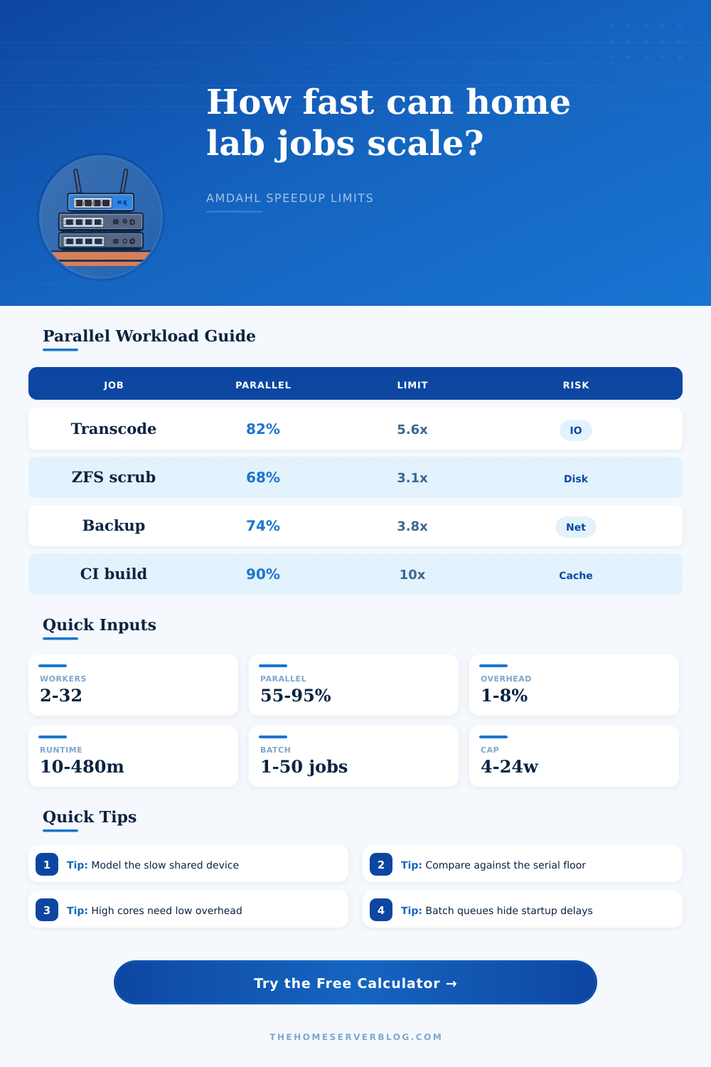
Amdahl Law Speedup Calculator
Estimate how far extra cores, worker threads, disks, or runners can accelerate home lab jobs before the serial portion and shared bottlenecks take over.
| Parallel Share | Serial Floor | Hard Speedup Limit | Home Lab Meaning |
|---|---|---|---|
| 60% | 40% | 2.5x | More workers help briefly, then orchestration dominates. |
| 75% | 25% | 4.0x | Good for backup, checksum, and mixed disk jobs. |
| 90% | 10% | 10.0x | Strong compile, encode, and independent queue scaling. |
| 97% | 3% | 33.3x | Only realistic when tasks are nearly independent. |
| Workload | Likely Serial Part | Shared Limit | Scaling Note |
|---|---|---|---|
| Video transcodes | Demux and mux | GPU session or disk read | Great until the media disk or encoder queue is full. |
| ZFS scrub | Metadata walks | Slowest vdev | Extra CPU does little once disks are saturated. |
| Backups | File listing | NAS write or network | Compression threads may outrun a 1 GbE link. |
| VM boot storm | Init ordering | Storage IOPS | More guests increase queue depth and lock contention. |
| CI builds | Dependency setup | Cache and test DB | Parallel runners shine when artifacts are isolated. |
| Scenario | Worker Range | Parallel Share | Practical Ceiling |
|---|---|---|---|
| Mini PC media node | 4 to 8 cores | 78% to 88% | GPU sessions or thermal headroom. |
| Four-bay NAS scrub | 4 disks | 55% to 70% | Slowest disk and metadata layout. |
| Proxmox cluster start | 6 to 18 VMs | 65% to 80% | Shared boot disk IOPS. |
| Self-hosted build pool | 4 to 24 runners | 85% to 94% | Artifact cache and test services. |
| Efficiency | Signal | Next Check | Home Lab Action |
|---|---|---|---|
| Above 70% | Healthy scaling | Thermals and memory | Add workers if the queue is consistently long. |
| 40% to 70% | Mixed scaling | I/O wait and lock time | Tune chunk size before adding more cores. |
| 20% to 40% | Bottlenecked | Disk queue and network | Fix the shared device or reduce concurrency. |
| Under 20% | Serial dominated | Startup and metadata | Batch jobs differently instead of scaling workers. |
More processors must be better, right? More cores mean faster jobs. Perhaps this is why you purchase a new server that has 32 threads of processing. Surely it will complete your backup routine in no time at all. But reality can bite back. While waiting for the CPU to catch up, the disk queues fills and cause the CPU to sit idle.
Amdahl’s Law represents the gap separating theory from throughput. It will help you adjust your expectations regarding parallel scale-out based off your own lab. It’s easy math. Getting it requires practice because there are problems in real systems not captured by raw clock speeds. That’s the core principle: finding the serial part of the work. This is the portion that cannot be parallelized or split into chunks, regardless of how many worker are used.
Why More Processors Do Not Always Mean Faster Speed
For video transcoding, it could be dealing with metadata headers or demuxing the stream(s). They have to occur in sequence first, then you can do the big lifting. Whether you apply one worker or eight workers, if twenty percent of job is serial, you’ll cap out at five times the speed. That’s the ceiling. And once people understand that ceiling, they won’t get caught in a never-ending upgrade cycle, buying more hardware while getting less and less return.
Model the scenarios with that overhead in mind: managing all those threads brings its own overhead. You need to lock shared resources and schedule context switches between them. For every extra thread in your pool, you pay an extra cost that grows at the same rate as the number of workers. Overhead on each single thread sounds like no big deal. But when multiplied over a huge batch, it can add up.
The calculator will crunch these numbers for you as soon as you specify both the size of the resource set and your desired parallel share, so you don’t have to guesstimate what fraction of time is spent coordinating. It forces you to think about system as a whole instead of just adding up core potential one by one.
In the home environment especially, storage bottlenecks tend to be the hard limit different than processing power. Whether it’s a crowded network interface or a single SATA drive, this becomes a funnel that limits parallel streams. Classic examples are a ZFS scrub or database indexing; they’ll saturate IOPS on disk long before running out of CPU cycles. Increasing the number of workers on an I/O bound task doesn’t make them go faster, it just adds depth to the queues, with longer wait times for each thread. The page offers some reference grids that lay this out, so you can see what kind of constraint you’re under (computational or infrastructural) and buy accordingly. If it’s the latter, knowing what device is handling the load lets you buy the right kind of performance, rather then the wrong one.
One exception is batch processing: since you’re amortizing the cost of starting up multiple jobs, it’s not as if you’re running them in parallel (unless your batch size is very small), but they do tend to smooth out any serial delays, so while one large task might expose serial delays that dominate total time, running fifty smaller tasks can hide those delays within the aggregate throughput. The tool actualy allows for specifying a batch size and will show how much faster things get when looking at real wall-clock time vs. Just speedup-per-job. That makes all the difference when you’re working with media libraries or a CI pipeline, where sheer volume is what counts more than speed of a single file. And what you want to optimize for isn’t how fast you can make it go at its best on some one-off unit of work, you need to optimize for total time from start to finish.
Mistakes include skipping over the serial floor altogether, or thinking it scales perfectly linearly forever. It takes 4 hours on a 4 core machine so it’ll be 2 hours on an 8 core. No! You have shared resource competition & fixed overhead. That’s why the efficiency metric in the results is there: it measures how effectively you’re using your resources. As you exceed the saturation point, efficiency drops. Once efficiency gets down under 40%, adding more hardware would of probably just be wasting power and money. Better to upgrade the shared bottleneck, or tune the workload instead.
Amdahl’s Law doesn’t mean we should avoid ambitious projects, it’s simply about spending wisely. It tells us when additional cores is useful and which ones will merely warm your room. Quantify the serial fraction and consider realistic penalties. This will let you estimate the benefits of adding more compute with decent accuracy. The result is operating smoothly within physical constraints instead of against them. When you acknowledge the limitations set by serial workloads, you no longer chase illusions… Instead, you optimize what matters. That enlightenment makes the hardware maze digestible as a system design problem.