Erasure Coding Calculator
Estimate K+M shard layouts, raw capacity, usable capacity, parity overhead, fault tolerance, and rebuild read amplification for generic erasure coded storage.
⚙Generic EC Presets
🧮Storage Inputs
📊EC Scheme Grid
📘Reference Tables
| EC Scheme | Minimum Devices | Usable Efficiency | Parity Overhead |
|---|---|---|---|
| 2+1 | 3 | 66.7% | 50.0% of usable |
| 4+2 | 6 | 66.7% | 50.0% of usable |
| 6+2 | 8 | 75.0% | 33.3% of usable |
| 8+2 | 10 | 80.0% | 25.0% of usable |
| 8+3 | 11 | 72.7% | 37.5% of usable |
| 10+4 | 14 | 71.4% | 40.0% of usable |
| Parity Shards | Shard Loss Tolerance | Best Fit | Planning Note |
|---|---|---|---|
| M=1 | 1 shard | Scratch or cache | Fastest and least protective |
| M=2 | 2 shards | General NAS data | Common balance of efficiency and safety |
| M=3 | 3 shards | Archive pools | Better during long rebuild windows |
| M=4+ | 4+ shards | Large cold pools | Higher overhead, stronger tolerance |
| Data Shards K | Rebuild Read Amp | One 18 TB Shard at 70% | Operational Impact |
|---|---|---|---|
| K=3 | 3× | 37.8 TB read | Lower read fanout |
| K=6 | 6× | 75.6 TB read | Moderate read fanout |
| K=8 | 8× | 100.8 TB read | Higher network load |
| K=12 | 12× | 151.2 TB read | Plan longer rebuilds |
| Workload | Suggested Direction | Capacity Bias | Rebuild Bias |
|---|---|---|---|
| Cold archive | More K, more M | High | Accept slower rebuilds |
| General files | 6+2 or 8+2 | Balanced | Moderate reads |
| Media library | 8+2 or 8+3 | High | Sequential friendly |
| VM and small files | Lower K or mirrors | Lower | Prefer faster recovery |
💡Planning Tips
You protect your data by splitting files into shards and scattering them among drives using erasure coding. The calculator show you what the rebuild timelines and capacity will look like. It removes the most common way storage projects go wrong: balancing efficiency and safety.
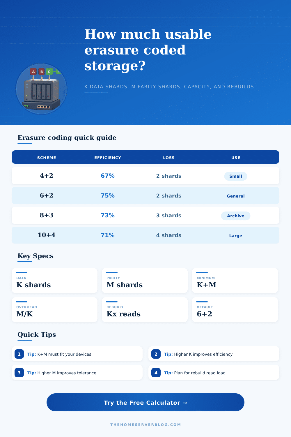
Selecting the right K and M values are essential. K is the number of data shards and M is the number of parity shards. Most people start with a 6+2 setup, meaning there are two parity shards and six data shards. That nets out at 75 percent efficiency; you get one-quarter less usable capacity, but you can withstand the loss of two hard drives simultaneousy. When you bump up to an 8+2 scheme, that boosts efficiency to 80 percent.
How to Choose the Right Settings for Your Storage
You save some space, but things change when a drive fail. You need to understand what happens in that event. To reconstruct the lost data, all the other data shards must be reread to recreate the missing bits. It’s called read amplification. When you lose a drive, the system reads through all surviving drives to reconstruct it. Things get bad if you have a high K value (12+). Your system will re-read terabytes of data to recover just one lost drive. How much? That depends on how full your drives are and their sizes. The calculator takes into account both factors and give a guess on how loaded your recovery might be.
For big pools with days-long rebuild times different than hours, this can also become a network bottleneck. You should also consider the type of data being stored: Virtual machines or hot databases requires a faster rebuild since their degraded performance will affect workloads. Backups that might remain untouched for months (cold archives) is less sensitive to slower rebuild times and can afford more parity overhead.
As you see from the reference table below, different levels of M corresponds to different degrees of risk tolerance. Higher parity provides greater safety with lower usable capacity. Lower parity are more efficient but has a slimmer margin. No free lunch in storage engineering.
Administrators also tend to overemphasize raw storage capacity without considering operating costs for maintaining it. In pursuit of maximum storage (every terabyte counts!), they stack drives together in tight configurations. Next thing they know, one bad drive bring down their fast network. That’s where steady rebuild speed comes into play; you’ll use it to model how much rebuilding will slow things down. A large K scheme may be too slow if your network can only sustain a rebuild rate of 350 megabytes per second.
Decide: Do you want maximum capacity? Or do you want maximum uptime? Determining the appropriate reserve percentage also matters. A typical value is leaving 10-20 percent of usable space in reserve to account for minor variances and metadata. This is your buffer against how people use the system in reality. If you don’t have that reserve, the system will feel full but actualy isn’t, resulting in wasted IOPS and unnecessary migrations.
There’s a tradeoff between resiliency and efficiency for erasure coding. There isn’t an option where you get both maximum resilience and maximum efficiency in the same setup. Your workload decides; the calculator give you the numbers. Use the presets as a starting point to examine how various schemes work on equivalent hardware limits.
Pay attention to rebuild read amplification because it hides some of the cost. After seeing these tradeoffs, choosing a K+M ratio becomes more of a calculated decision then a guess. It’s about building a storage pool that stores data without wasting resources or compromising security. You should of checked the numbers first.