Cascaded Return Loss Calculator
Estimate effective return loss for a chain of RF, coax, Ethernet, or bench-test discontinuities by combining each stage reflection with the insertion loss ahead of it.
Each stage contribution is converted from return loss to reflection coefficient, then reduced by twice the insertion loss before that point. This estimates how loudly each discontinuity echoes back to the source.
Stage-by-Stage Breakdown
| Effective return loss | Equivalent VSWR | Reflected power | Typical interpretation |
|---|---|---|---|
| 30 dB or better | 1.07:1 or lower | 0.10% or less | Excellent bench termination, precision adapter stack, or calibrated reference path. |
| 24 dB | 1.13:1 | 0.40% | Strong source-facing cascade for most home lab RF and receive chains. |
| 20 dB | 1.22:1 | 1.00% | Good practical target for quality coax jumpers, filters, and antenna ports. |
| 14 dB | 1.50:1 | 3.98% | Often acceptable for many antenna systems but can be weak for sensitive links. |
| 10 dB | 1.92:1 | 10.00% | Marginal cascade; inspect the worst discontinuity before blaming the radio. |
| 6 dB | 3.01:1 | 25.12% | High reflection risk, especially with power amplifiers or wideband data links. |
| Stage type | Common source of reflection | Useful data-sheet value | Cascade note |
|---|---|---|---|
| Connector pair | Pin depth, wear, plating damage, water ingress | Return loss or VSWR at frequency | Early connector reflections are not attenuated by much path loss. |
| Adapter | Geometry transition and impedance step | Return loss plus insertion loss | Stacked adapters can dominate even when each looks acceptable alone. |
| Filter or arrestor | Port match changes near passband edge | S11 and S22 across the operating band | Use the worse port if direction is unknown or reversible. |
| Feedline section | Crush, bend radius, moisture, poor shield contact | Return loss and attenuation per length | Its own reflection may be small, but its loss masks later echoes. |
| Antenna or load | Actual resonance, mounting, nearby metal, weather | Measured return loss at installed band | Often the largest raw reflection, but feedline loss may reduce what the radio sees. |
| Profile | Nominal impedance | Planning target | Where it fits |
|---|---|---|---|
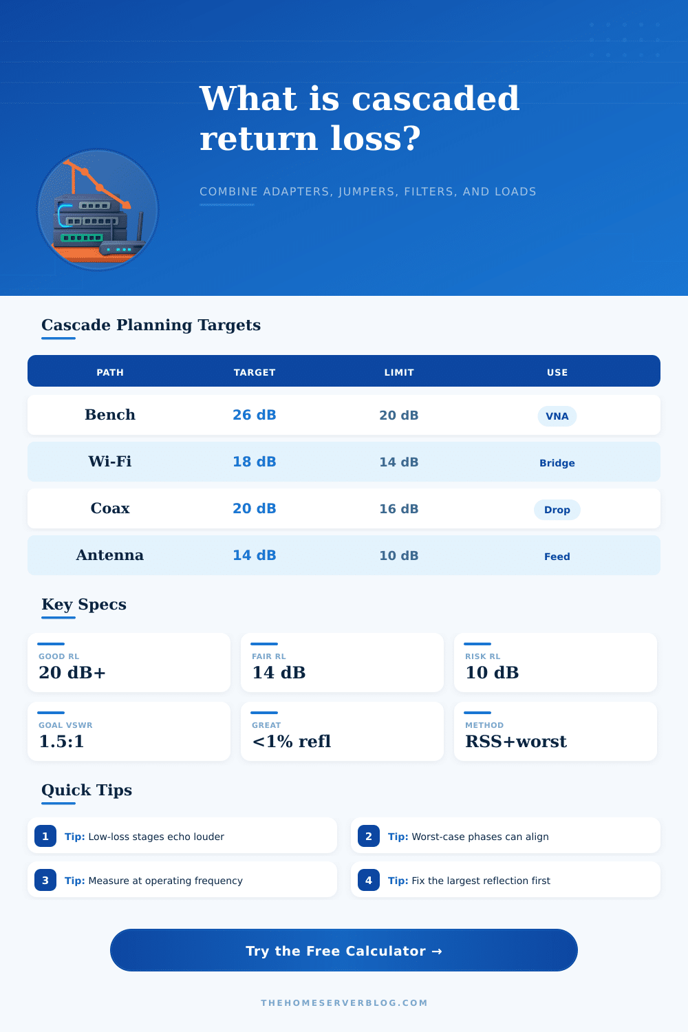
| 50 ohm RF coax chain | 50 ohms | 18 to 20 dB | Wi-Fi, LoRa, SDR, amateur radio, lab instruments, and outdoor antenna feeds. |
| 75 ohm coax distribution | 75 ohms | 16 to 20 dB | DOCSIS, satellite, video distribution, splitters, and terminated coax drops. |
| 100 ohm Ethernet channel | 100 ohms differential | 12 to 18 dB | Patch panels, keystones, modular plugs, cable bends, and balanced-pair channels. |
| Precision bench path | 50 ohms | 26 dB or higher | VNA calibration checks, attenuator stacks, filters, switches, and reference loads. |
| SFP+ DAC twinax | 100 ohms differential | 15 dB or higher | Short passive rack links where plug transition quality affects eye margin. |
| Project example | Typical stages | Result to watch | Practical fix |
|---|---|---|---|
| Outdoor LoRa gateway | Radio port, adapter, arrestor, feedline, antenna | Final load plus arrestor reflections | Move to fewer adapters and check antenna match after mounting. |
| 5 GHz bridge | PoE radio pigtail, SMA adapter, coax, panel antenna | Small losses but many connector transitions | Use one proper jumper instead of multiple short adapters. |
| DOCSIS service drop | Tap, splitter, wall plate, modem cable, modem port | 75 ohm mismatch at open ports | Terminate unused splitter ports and replace damaged F connectors. |
| SDR filter stack | Receiver, attenuator, filter, switch, preamp, antenna | Bench adapters near the receiver | Keep precision adapters close to the VNA and sweep the full band. |
| Cat6 patch channel | Patch cord, jack, horizontal cable, patch panel, switch | Near-end return loss | Preserve twist to the termination and avoid tight bends behind panels. |
This calculator estimates linear cascade behavior for planning. Final compliance or production work should use calibrated VNA measurements, correct port extensions, fixture de-embedding, and frequency-specific component data.
When you builds an RF path, you add various component: connectors, adapters, and lengths of cable. Every connector, every adapter, and every length of cable adds a reflection to the RF path. Each reflection does not remain at the location where the reflection is created; it travel back to the source.
As the reflection travels back to the source, the reflection weaken due to the loss along the path that the reflection takes to return to the source. The total amount of reflection that falls into the radio or the RF instrument is the value of interest. This value is called the cascaded return loss for the RF path, and the cascaded return loss value is rarely the same then the lowest return loss value for any of the components along the path.
How Return Loss Adds Up in an RF Path
The cascaded return loss are difficult to manage because the reflection with the lowest return loss value is not necessarily the worst reflection along the path. For instance, a mediocre quality connector placed near the radio will produce a stronger reflection than a poor quality antenna placed at the end of the RF path behind several meter of cable. The loss of the cable has two jobs: to attenuate the signal traveling out of the radio to the antenna, and to attenuate the reflection traveling from the antenna back to the radio.
The attenuation of the reflection by the cable mean that the value of the return loss of a component located miles from the source will not have a strong effect on the source. A calculator can help with the math involved in determining the cascaded return loss, thus removing the need to guess how much loss will attenuate each reflection along the path. While return loss is a value that describes the size of the reflection coefficient, return loss does not describe the behavior of reflection coefficients when placed in series with each other along an RF path.
The reflections add together coherently or incoherently depending upon their phases; the phase relationship between the reflections shift as the cable shifts or changes temperature. Thus, the calculator includes methods for combining the return loss values along the RF path. One method for combining return loss values is a planning blend, which creates a conservative estimate for cascaded return loss because it does not assume that each reflection arrive in step with each other along the path.
An alternative method for calculating cascaded return loss along an RF path is the RSS approach, which creates a result that is typical of the RF path and closer to the measurements that are obtained from an RF path whose components is moving. The method chosen has an impact upon the margin that can be allowed in the RF path prior to installing the hardware for that path. Each of the inputs to the calculator has an impact upon the RF path that will be created.
The reference impedance is the baseline for each component along the path, and each component along the path can be judged relative to this baseline. The frequency of the RF path set the length of the electrical path along the path, and the frequency impacts how much shift in phase occurs with small shift in physical position of the cable. The buffer percentage accounts for many factors along the path; the buffer percentage accounts for the aging of the connectors, the buffer percentage accounts for the number of mating cycles performed on the connectors, and the buffer percentage accounts for the difference between laboratory measurements of RF components and the real world (such as wind, water, and other factor that alter the performance of the components).
While the numbers for each of these variables dont need to be perfect, the numbers for each of the variables must be honest in their description of the parameter for the RF path that will be created. While the calculator can provide an estimate of the performance of an RF path based off the return loss of its components, the calculator does not take into account the physical layout of the RF path. Components with the same return loss values will have different impact upon cascaded return loss based upon the physical positioning of those components along the RF path.
For instance, a component with a high return loss value placed near the source will have less attenuation of its reflection than a component with a high return loss value but placed miles from the source. Thus, the first few components along the RF path will have a greater impact upon cascaded return loss than the components placed near the antenna. Fixing the first connector or the first adapter will have a more greater impact upon cascaded return loss than replacing the antenna, even if the return loss of the antenna is worse.
The calculator shows which stage along the path create the largest weighted return loss for the RF path; this information is often missed by those who only review the return loss of each component along the path. The calculator assumes linear behavior at a single frequency along the RF path. The RF path will likely include many different frequency band.
A component like a filter or an antenna may appear to have a good return loss at the center frequency of a band, but the performance of that component may degrade at the edges of the frequency band. Additionally, changes in temperature will impact the velocity factor of the coaxial cable along the path; the repeated flexing of the cable will impact the electronic match of the connectors along the path. Each of these effect is beyond the consideration of the calculator; the output of the calculator is a planning target for the RF path.
If the calculated cascaded return loss is several decibel above the requirement for return loss, there will be margin for real world effects. If the calculated cascaded return loss is nearly at the requirement for return loss, it is likely that measurements of the completed RF path will be performed to ensure that it is finished correctly. The reference tables located on the page allow for the final numbers for the cascaded return loss to be translated into a more usable format.
Each of the reference tables indicate the implications of different return loss values regarding reflected power and VSWR for the RF path. Additionally, each of the reference tables associate common type of components along an RF path with the problems that are common with those type of components. While the reference tables dont need to be memorized, it is important for those who calculate cascaded return loss to recognize when the calculated value indicate that small improvements will make a big impact upon the RF path; it is also important to recognize when the cascaded return loss as calculated is already good enough that further effort will not greatly increase the performance of the path.
Overall, the calculation of cascaded return loss is a method for those who plan to construct an RF path to ask the question of whether the RF path will be acceptable before the RF path is constructed. By describing each of the components that will be used along the RF path, the cascaded return loss calculator will provide an estimate of the return loss that will be experienced by the source or radio. The margin that is required indicate whether the calculated return loss will be acceptable.
Thus, the calculation requires some measurement and judgment of the components that will be used; however, it do provide a clearer picture of which of the components along the RF path will contribute to the formation of the loudest reflection within that RF path.