HomeServerBlog analytics storage tool
Column Storage Calculator
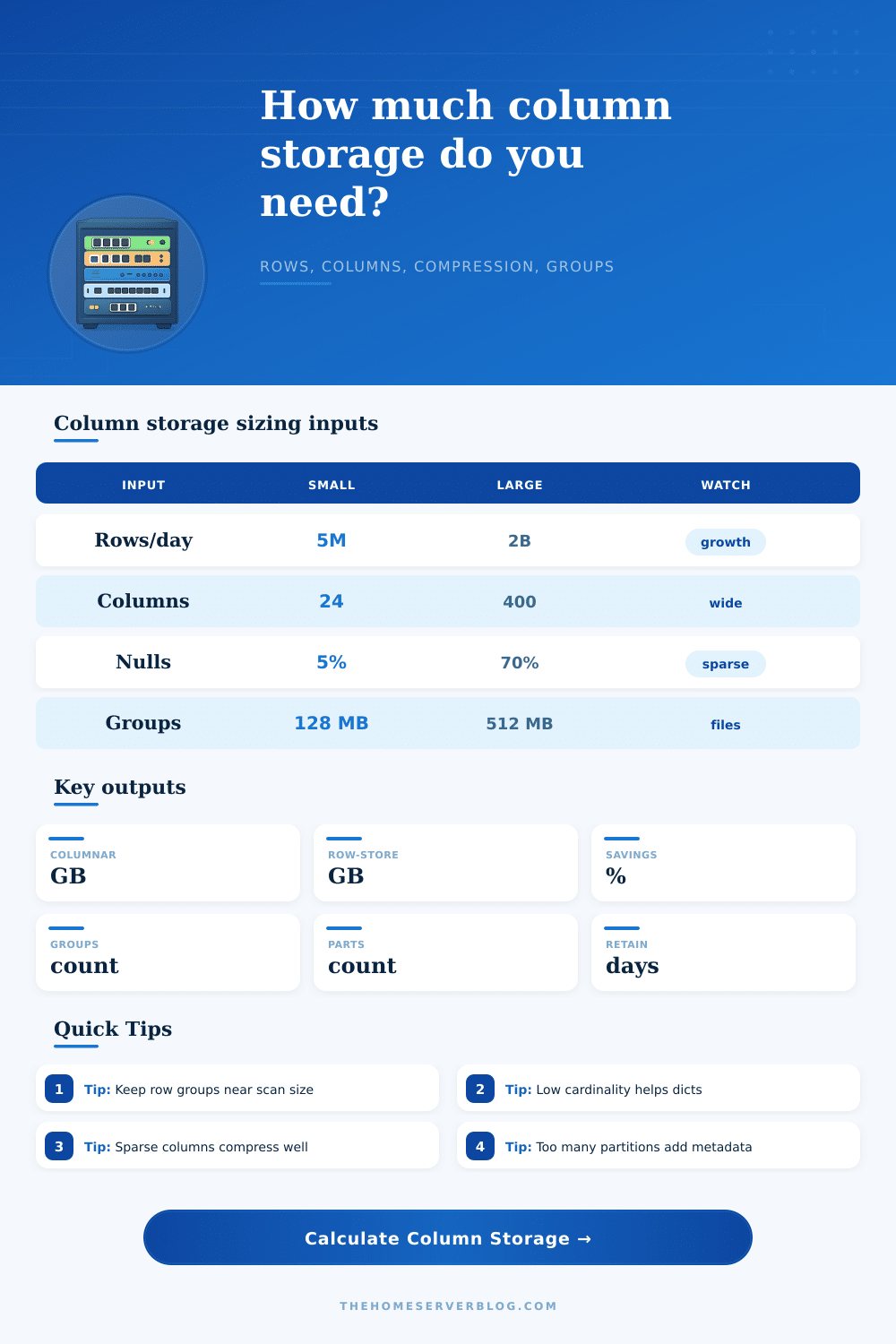
Estimate retained columnar storage from rows, columns, average column bytes, compression ratio, dictionary cardinality, null density, row group size, partitions, metadata overhead, and retention.
Total row and column positions before null pruning.
Cardinality as a share of rows per row group.
Higher values usually scan better than tiny partitions.
Footers, marks, manifests, and partition tracking.
Parquet
128-512 MBColumn chunks, row groups, statistics, and strong compatibility across lakehouse query engines.
ORC
64-256 MBStripes, indexes, bloom filters, and efficient compression for Hive-style fact tables.
ClickHouse
Parts + marksSorted parts, marks, primary key ranges, and merge behavior shape storage overhead.
DuckDB
Row groupsLocal analytics files benefit from compact row groups and typed columns on disk.
BigQuery Export
Columnar filesExports often land as Parquet or Avro, where partition count and schema width matter.
| Formula piece | Calculator logic | Raises storage | Lowers storage |
|---|---|---|---|
| Retained rows | Rows per day multiplied by retention days | Higher ingest or longer retention | Lifecycle expiry or rollups |
| Row-store comparison | Retained rows times column payload plus row header and null bitmap | Wider rows and low null share | Fewer columns and sparse values |
| Columnar data | Non-null column payload divided by adjusted compression ratio | High cardinality or weak compression | Low cardinality, nulls, and good row groups |
| Metadata overhead | Percent overhead plus row group stats and partition manifests | Small row groups and many partitions | Larger row groups and coarser partitions |
| Dictionary cardinality | Density in row group | Expected effect | Planning note |
|---|---|---|---|
| Very low | Under 1% | Strong dictionary win | Status, region, enum, and category columns usually fit here. |
| Low | 1% to 5% | Good compression help | Product, device, and tenant columns may still benefit. |
| Medium | 5% to 25% | Mixed result | Check whether sorted data improves repeated runs. |
| High | Over 25% | Dictionary overhead risk | IDs, UUIDs, and free text may fall back to plain encoding. |
| Row group target | Typical use | Storage behavior | Query tradeoff |
|---|---|---|---|
| 16-32 MB | Small local tables and frequent writes | More footers and weaker compression | More parallelism, more metadata |
| 64-128 MB | Balanced Parquet and DuckDB analytics | Good compression and manageable stats | Works for many BI scans |
| 256-512 MB | Large fact tables and cold partitions | Strong compression, fewer groups | Selective queries may read larger chunks |
| Over 512 MB | Long scans and archive-style reads | Low metadata share | Can reduce parallelism for smaller engines |
| Preset | Data shape | Storage pressure | Best tuning lever |
|---|---|---|---|
| Parquet Metrics Table | Narrow typed metrics with regular dates | Row groups and compression ratio | Keep groups near 128 MB and sort by time. |
| ORC Data Lake Fact | Large fact table with dimensions | Retention and partition count | Use coarse partitions and strong stripes. |
| ClickHouse Events | High event rate with sorted parts | Part metadata and merge pressure | Choose order keys that improve runs. |
| DuckDB Local Analytics | Local file for notebook or desktop BI | File size and row group balance | Avoid too many tiny partitions. |
| BigQuery Export | Exported warehouse slices | Wide schema and metadata | Project only needed columns before export. |
| Sparse IoT Columns | Many optional sensor fields | Null maps and partition fanout | Group devices or metrics to avoid tiny files. |
| Wide Audit Table | Many nullable compliance fields | Metadata and wide schema stats | Separate rarely used blobs from typed fields. |
| Product Catalog Columns | Repeated categories and attributes | Dictionary cardinality | Normalize noisy names and enums. |
| Time-Series Rollup | Aggregated counters and timestamps | Retention more than raw bytes | Roll up old buckets and keep sorted time ranges. |
How many bytes do I need? That’s the first question people ask when they sit down to design their data lake. Sounds straightforward, right? Until you learn that most raw byte counts is a trap. A table may appear to require two terabytes of storage, yet half of that will vanish when compression sets in. Here’s the twist: What are we really measuring? And does the way we lay out our tables matches our query patterns?
Most teams begin with row and column count. That’s great for a ballpark estimate. However, storage engineering becomes serious when you think about how those values combine on disk. Volume without time is meaningless; row count without context isn’t helpful.
How to Plan Your Data Storage
The tool will even figure out the coefficients and conversions for you, so that you don’t have to guess or do any math. And it lets you see efficiency in columns. What’s the average bytes per column value? How many rows can you fit into a gig?
It begins with rows per day and retention days, since those define your volume. Your storage footprint will double if you store data for six months rather than three, no matter how cleverly design your schema.
You then must consider the average bytes per column value. It is not the max string length of some field, but what the typical record realy looks like on disk. Next is compression, which people often confuse or get excited about. Compression really shines when columns is grouped together (e.g., in columnar formats such as ORC or Parquet). Dictionary encoding will crunch values of the same kind down to small pointers. If you have a status column with just four different statuses, those gets crushed down to tiny pointers.
That’s where the number of unique values in the dictionary gets fed back into the calculator, so it knows how many bytes those dictionaries take up and how many bytes they’re saving over raw data. Low cardinality is your friend. UUIDs and user IDs don’t generally benefit from dictionary compression; high cardinality isn’t usually helpful. So the tool changes the ratio according to what you feed it instead of assuming some universal multiplier apply across all things.
How dense are your nulls? More than you’d think. Since every row include its own header and padding, a row store often uses as many bytes for nulls as it does for actual data. Columnar stores can marks nulls with a lightweight bitmap, or skip them altogether. The calculator does this by considering that null-heavy columns mean a smaller effective payload. If you set it up correctly, you’re not paying for empty space, particularly helpful on wide audit tables or IoT feeds where maybe not all metrics get reported every time interval.
Another lever affecting performance and storage space is row group size. Smaller sizes means better query detail (less data to skip). However, a larger size mean more metadata and footer overhead. And the trade-off between those two are illustrated nicely in the reference table on the page: too small and you get an explosion in maintenance burden from all your little partitions; too big and it may harm query parallelism. So there’s a sweet spot in the middle I guess. For a balanced workload, typically 128 to 512 megabytes per group does the trick. This provides enough data to allow compression algorithms to pick up some patterns, but not so much as to force scanning an entire day’s worth of history to recover a single timestamp.
Metadata overhead is often overlooked. Index structures, statistics, headers, and more is required for each column chunk. They are also required for each row group and partition. You has thousands of small files because you partitioned by tenant and hour? And each has a footer. Those footers add up fast. The calculator has a metadata percentage field so you can model this out explicitly.
Splitting your data out does make it faster; true enough for pruning purposes. But if you wind up with more metadata than actual payload, then you’ve lost the battle before it started. It provides an output that shows you how many rows stores would save you compared to what you have now. So it shows you if you are using storage efficienty, or how much space you could save by changing your layout.
The verdict section tells you if your design is well balanced. Is there too much shared metadata? Consider grouping more broadly. Is the dictionary not dense? Are there a lot of repeating values in your columns that could be stored compactly with encoding?
There is no such thing as best size in storage planning. It’s about matching your design to how you want to use the data in the future. To summarize, storage architecture is not a numbers game; it’s a structure game. You are looking for layouts that play nicely with your query patterns while minimizing administration overhead.
Begin with an estimate of your daily ingestion rate, what do you think is realistic? Tweak the retention policy to find the size that matches your budget. Modify the partitioning strategy to reduce metadata. Once you get the geometry right, the storage cost will follow naturaly. That’s kind of the whole reason we moved past flat row files in the first place.