Disk RAID and IOPS Calculator
Estimate usable capacity, random read and write IOPS, parity penalty, cache effect, and rebuild reserve for a NAS, VM datastore, or home lab storage pool.
Calculation Breakdown
| RAID Level | Minimum Drives | Usable Capacity Rule | Random Write Penalty | Best Home Server Use |
|---|---|---|---|---|
| RAID 0 | 2 | N drives | 1x | Scratch data, temporary media work, no redundancy |
| RAID 1 | 2 | 1 drive | 2x mirror write | Boot pools, two-bay NAS, important small datasets |
| RAID 5 / RAIDZ1 | 3 | N minus 1 drive | 4x parity write | Small arrays with backups and moderate writes |
| RAID 6 / RAIDZ2 | 4 | N minus 2 drives | 6x parity write | Large HDD NAS pools, backup shelves, archive storage |
| RAID 10 | 4 | Half of total raw capacity | 2x mirror write | VM storage, databases, mixed read/write home labs |
| RAIDZ3 | 5 | N minus 3 drives | 8x model estimate | Very wide ZFS pools where rebuild risk dominates |
| Drive Class | Read IOPS | Write IOPS | Latency Character | Calculator Use |
|---|---|---|---|---|
| Archive HDD | 55-80 | 45-70 | High seek latency | Backups, media archives, cold storage |
| 7200 RPM NAS HDD | 75-110 | 65-100 | Moderate random IO | Home NAS, media, general file share |
| Enterprise 10K HDD | 130-180 | 110-160 | Better seek time | Legacy servers, lighter VM pools |
| SATA SSD | 70000-100000 | 50000-90000 | Low latency | VM datastore, app data, metadata special vdevs |
| Enterprise SATA SSD | 90000-110000 | 70000-100000 | Steadier sustained writes | Sync-heavy services and databases |
| PCIe NVMe SSD | 400000-1200000 | 250000-900000 | Very low latency | Fast VM hosts, build servers, cache tiers |
| Workload | Typical Mix | Queue Behavior | Cache Impact | Planning Note |
|---|---|---|---|---|
| SMB/NFS file share | 60-80% reads | Moderate bursts | Helpful for repeat reads | Balanced settings usually match a family NAS |
| Virtual machines | 50-70% reads | Random and parallel | Helps boot storms | Write latency matters more than peak read IOPS |
| Database or sync writes | 40-70% reads | Small synchronous IO | Limited without safe write cache | Prefer mirrored SSD or RAID 10 |
| Media streaming | 90%+ reads | Sequential | Can be very helpful | Capacity and throughput often beat random IOPS |
| Backup target | Write-heavy bursts | Large sequential writes | Read cache is minor | Parity arrays are acceptable when windows are long |
| Surveillance ingest | Mostly writes | Steady sequential streams | Low value | Use drive workload ratings and free-space reserve |
| Scenario | Array Example | Capacity Result | IOPS Character | Practical Fit |
|---|---|---|---|---|
| Two-bay NAS | 2 x 8 TB RAID 1 | 8 TB before reserve | Good reads, single-disk writes | Documents, photos, light media |
| Four-bay media NAS | 4 x 12 TB RAIDZ1 | 36 TB before reserve | Read-friendly, parity write cost | Media libraries with backups |
| VM lab datastore | 6 x SSD RAID 10 | 50% raw before reserve | Strong mixed random IO | Proxmox, ESXi, Hyper-V labs |
| Backup shelf | 8-12 HDD RAID 6 | N minus 2 drives | Good reads, slower random writes | Snapshots, backups, cold datasets |
RAID is not a backup. The calculator estimates array behavior, but it does not account for accidental deletion, ransomware, controller faults, bad snapshots, or offsite recovery needs.
For many home server geeks, it begins here. Order a four-bay case. Populate it with some matching drives. Watch them blink. Attempt to use your system. Booting up a virtual machine feel sluggish. Streaming two shows simultaniously seems slow. On paper, this setup appears fine. In reality, it is slowed down by the number of read and write operation per second. You don’t learn enough that RAID isn’t only about storage space, it’s about how data moves across components, especially in stressful situations.
Once you’ve entered in your workload mix and drive count, the calculator above do the rest of the work. You don’t have to guess anymore if your parity array will support those midnight backups.
Why Your Home Server Is Slow
When most folks construct a storage pool, all they think about is terabytes. That’s understandable; the only thing written on the box is capacity. What happens behind the scenes when the operating system ask for a single small file determines performance. The stress is measured by random IOPS, which tell you just how many separate request your drives can respond to per second without queueing up. Even though your sequential bandwidth might look fine, if your random writes are low, your system will seem slow.
You should of understand the parity penalty. When you write to a RAID 5 or RAID 6 array, the controller cannot just dump bytes onto disk. It needs to read the old block, calculate the new parity information, and then write the data plus the parity back. That’s a read-modify-write cycle that hurt random write performance on traditional spinning hard drives. To account for the additional mechanical work, the calculator multiplies its numbers by something that represents that penalty. If you’re doing a general file share where reads dominate, it isn’t too bad. But if you’re hosting virtual machines or running a database, all those little writes will choke the array. For performance critical workloads, mirrored configs tend to win here because they perform writes better, even though they use half of your raw capacity for redundancy.
It also adds a layer of complexity that most builders miss: cache behavior. When your most frequently accessed data resides in fast memory (cache) instead of hitting the physical drives, it creates high cache hit rate that dramatically reduces the IOPS demand on your storage pool. This results in a higher cache hit rate. For example, if you’re doing media server, chances are that your users will be watching same popular shows over and over again. The cache easily absorbs those hits. However, if you’re doing a surveillance feed or a backup job, you generate unique data every second. There’s nothing repeating itself, so there’s nothing getting cached. Every time, your drives has to do all the work. Understanding this difference will help you set realistic expectations around latency and throughput based off how users behave.
The one thing that gets ignored in today’s storage planning is rebuild reserve. We have huge drives these days. Twelve or sixteen terabytes on a single drive isn’t uncommon. In an array of drives, if one goes bad, rebuilding the missing data onto a spare disk can take days. And once it’s down, there’s a strong statistical chance that something else will fail while it’s down. Having some free space means your filesystem can keep up with the update operations for its metadata and snapshots without falling behind. It gives you time to breathe when your storage is at its most vulnerable. Don’t ignore it, as one little hiccup could of go very wrong.
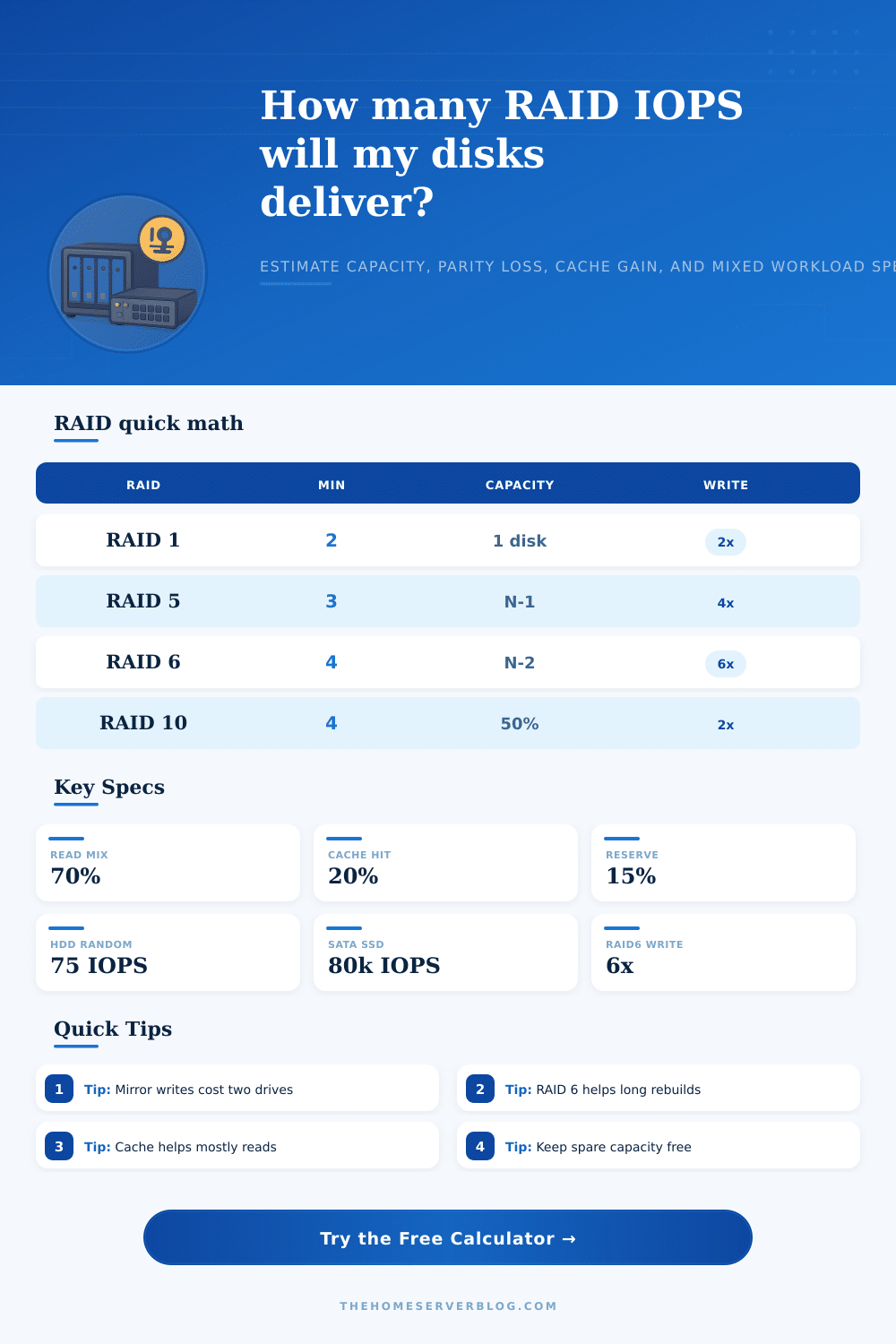
In the end it comes down to a trade-off between resource efficiency vs. Risk. Mirrors are easy/fast to write but burn through capacity fast. Parity arrays don’t waste space, but penalize random writes and have longer rebuild time than they should. In storage there’s no such thing as a free lunch. What matters most to you? Do you want the maximum amount of usable space, or consistency under load? The chart on the page breaks it all down nicely, comparing minimum drives required against how they are meant to be used.
Ultimately, it’s unobtrusive. Files open quickly, backups complete without getting in your way throughout the day. You’re reassured that you won’t lose all of your online life should one drive fail. With the calculator, before committing to buy drives, you’ll know if your array can handle your workload. It converts specs from abstraction to prediction. You’ll be able to see the tradeoffs, so that when your home server is as nice as it looks, it will perform just as well.