Elasticsearch Capacity Planning Calculator
Forecast storage growth, hot and warm tier pressure, heap demand, CPU headroom, and the month your cluster runs out of usable capacity.
Forecast breakdown
Hot-only
Best for small clusters and short retention. Forecast disk pressure directly against fast data nodes and leave extra reserve for segment merges.
Hot/Warm
Best for logs and observability. Keep recent data on fast disks, move older searchable data to denser warm nodes, and size each tier separately.
Replica-heavy
Best when read availability matters. Capacity multiplies quickly, so model replicas before ordering nodes or extending retention windows.
Growth-first
Best for fast ingest products. Monthly growth is compounded before retention capping, which exposes exhaustion month earlier than a flat daily estimate.
| Planning signal | Healthy range | Watch range | Action when exceeded |
|---|---|---|---|
| Disk after reserve | Under 75% | 75% to 90% | Add nodes, reduce retention, or improve compression before high watermark relocation starts. |
| JVM heap headroom | Over 30% | 15% to 30% | Reduce shard count, add data nodes, or split hot and warm tiers by workload. |
| CPU headroom | Over 35% | 15% to 35% | Separate ingest from search, add vCPU, tune refresh intervals, or reduce query fan-out. |
| Exhaustion horizon | 12+ months | 3 to 12 months | Plan capacity purchase, tier migration, or retention changes before operational pressure arrives. |
| Workload profile | Capacity driver | Typical compression | Planning note |
|---|---|---|---|
| Log analytics | Daily ingest and retention | 0.35x to 0.60x | Hot/warm sizing usually matters more than peak query concurrency. |
| Security events | Replica count and retention | 0.45x to 0.70x | Keep more reserve for incident surges and delayed ingest catch-up. |
| Metrics and traces | Cardinality and volume | 0.55x to 0.80x | CPU and heap pressure can arrive before disk fills. |
| Search application | Query concurrency | 0.65x to 0.95x | Read replicas may be capacity strategy, not just availability strategy. |
| Tier | Common role | Reserve target | Capacity planning focus |
|---|---|---|---|
| Hot | Recent writes and active queries | 20% to 30% | Fast disks, merge headroom, query concurrency, and ingest bursts. |
| Warm | Older searchable data | 15% to 25% | Dense disks, retention window, replica multiplication, and recovery time. |
| Cold or frozen | Rare access and archive | Varies by design | Search latency tolerance, cache size, and snapshot restore assumptions. |
| Coordinating | Query routing | CPU based | Not counted here; add separately when dashboards or aggregations are heavy. |
| Capacity lever | Storage effect | Heap effect | CPU effect |
|---|---|---|---|
| Reduce retention | High | Medium | Low to medium |
| Improve compression | High | Medium | Low |
| Add data nodes | High | High | High |
| Lower query concurrency | Low | Low to medium | High |
The common pattern with most Elasticsearch outages is that they begin slow. There’s no “explosion” of error reports, just disk usage creeping towards high watermark. Dashboards is slower as merge performance starts to lag. Shards aren’t being relocated quick enough, and writes is getting rejected by the cluster. The window to smoothly expand the cluster has long passed by the time anyone notify ops.
Capacity planning isn’t about purchasing additional hardware today; it’s about predicting when your architecture will fail tomorrow, so you can respond before alarm bells ring.
How to Plan Your Storage Needs
So what does it do? You provide your ingest rates (how much data goes into ES) and your retention target (how long you keep it). Then you let the calculator do the rest. No more guesswork about how replicas and compression build on each other over time.
The most common gotcha is compression factor as the first input to plug in. Log data appears large in its raw form, but then Elasticsearch puts it through different lens compared to a file system when storing. After segment merges and indexing are complete, text-heavy logs can shrink considerably. That means if you think raw volume = storage cost, then you’re going to overspend. Adjust this number to match your workload profile.
The tool recognize that not all JSON payloads are created equal, they don’t compress as well than plain text logs. The problem multiplies quick if there is replicas. A single replica has two copies of every shard, two replicas has three. Every copy eat up heap memory and disk space. And then when you model a cluster with high availability requirements, the storage triple (or doubled) instantly.
That’s where the calculator splits hot and warm tiers. Hot nodes are handling recent searches and active writes, which require lower latency and faster I/O. The warm node store older data. The priority here isn’t speed but rather density. You don’t want to pay for premium storage on data that rarely gets queried. By separating these, you can size each layer correctly based off its own.
Heap size is another quiet assassin. Keep it below thirty-two gigabytes per node. That is the point where Elasticsearch stop using the whole JVM heap effectively. Beyond that limit, it starts using compressed ordinary object pointers, which greatly increase the memory cost of a single reference. And when you have lots of concurrency in your queries, you’ll hit heap pressure since they’re going to need to load more field data structures and possibly more segments into the filter cache. The calculator take into account how much memory your concurrent query load demands from the heap, plus how large your primary size is. If it shows you’re running with low headroom, you probably don’t need more RAM per node, you probably need more nodes.
In search-heavy environments, it’s not usually disk that comes first; rather, it’s CPUs. Complex filters and aggregations can consumes cycles rapidly. To model CPU pressure, the tool takes into account workload profiles. For example, a static search index will stress a processor in different way from a metrics dashboard with thousands of time-series fields. This understanding allow you to choose between adding more vCPUs or splitting your workloads across separate managing nodes.
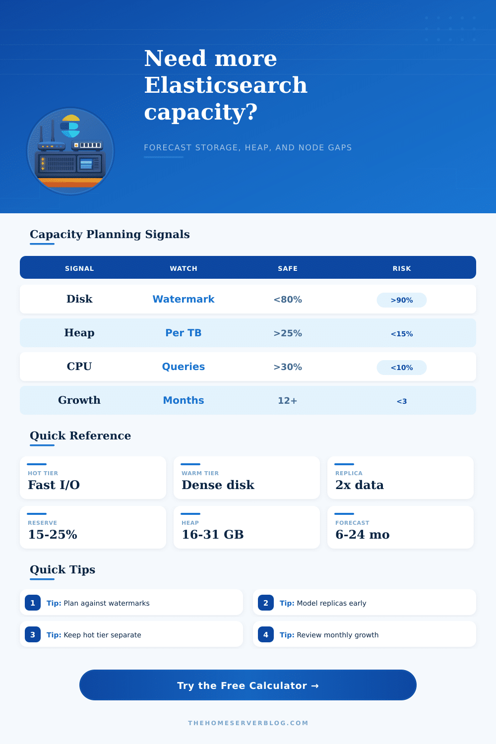
In the tool itself, there’s a set of reference tables explaining what’s considered normal (healthy) levels for CPU, heap, and disk use. These aren’t hard stops; they’re guidelines. Eighty percent disk use is fine for continued growth; ninety percent shows you want to relocate some data, but you can still do it safely. Having those as your watermarks lets you plan and provides you with wiggle room to deal with unexpected spikes and do routine maintenance.
It also lets you estimate the month you’ll run out of capacity, assuming nothing changes. That way, instead of panicking when it happens, you know when it’s coming so you can plan your purchase/architectural shift months in advance.
That’s what makes capacity planning an iterative process. Over time, your data will grow, your queries evolve, and your business priorities change. Regularly revisiting these inputs will make sure that your infrastructure keeps up with you, rather than holding you back. Better to build out a cluster slowly over time as you can test things, rather than scrambling in the middle of an incident.
Use the basics as a starting point, tweak it based off how many replicas and how much compression you use, and then let the prediction tell you where to go from there. It’s about keeping yourself stable, not just stashing away storage.