Home server and enterprise log sizing
Splunk Capacity Planning Calculator
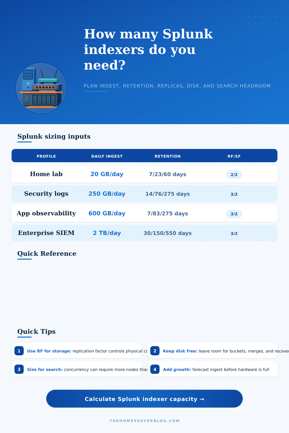
Estimate Splunk indexers, hot/warm/cold storage, ingest per indexer, replication overhead, search concurrency headroom, and search head guidance from practical sizing inputs.
Capacity breakdown
Constraint check
Lab indexer
8 CPU cores, 32 GB RAM, 1.2 TB usable disk. Best for small home lab, short retention, and light search activity.
Standard indexer
16 CPU cores, 64 GB RAM, 2.4 TB usable disk. A practical baseline for many log analytics clusters.
Large indexer
24 CPU cores, 128 GB RAM, 6 TB usable disk. Useful when search concurrency and daily ingest are both meaningful.
Storage dense
24 CPU cores, 128 GB RAM, 12 TB usable disk. Fits long warm or cold retention when searches are less frequent.
| Input | What it changes | Practical planning note |
|---|---|---|
| Daily ingest GB | Storage, CPU, parsing, indexing throughput | Use measured license or index volume, then apply the growth percentage. |
| Hot, warm, cold days | Storage per tier and search speed expectations | Hot handles active writes. Warm keeps searchable history. Cold is for slower retention. |
| Replication factor | Physical storage multiplier | RF 3 means three physical copies of bucket data across the cluster. |
| Search factor | Searchable copies and recovery posture | SF should be less than or equal to RF. The calculator flags values above RF. |
| Compression factor | Stored primary bucket size | Use a conservative value for noisy JSON, verbose Windows events, or indexed fields. |
| Concurrent searches | Indexer and search head sizing | Scheduled reports, dashboards, and ad hoc investigations all count at peak. |
| Tier | Typical use | What to watch | Calculator output |
|---|---|---|---|
| Hot | Recent data and active bucket writes | Fast disk, indexing load, frequent searches | Hot storage TB and hot share of retained data |
| Warm | Searchable retained history | Disk fill, bucket count, dashboard range queries | Warm storage TB and tier days |
| Cold | Longer retention on slower storage | Restore expectations, slower searches, archive policy | Cold storage TB and total retained days |
| Indexer pool | Cluster peers that store and search data | RF minimum, CPU, RAM, disk, search pressure | Recommended indexer count and limiting constraint |
How much do I need? Don’t worry, Splunk has a calculator for that. Enter your retention goals, along with your estimated amount of data coming in each day, and it does all the math for you; no more converting or guessing at numbers. It translates vague “I need this and this” statements into exact disk tier and server count number so you can begin building with confidence rather than guesswork.
It does not treat all data equally. Data isn’t treated as raw bytes; instead, certain types is compressed more or less than others by default (Splunk does this quite a lot). A long, verbose stack trace from Java are going to shrink down different than a small, tight CSV event. Unless you account for that with some kind of average compression factor, you’ll find yourself estimating and drifting away from reality.
How to Use the Splunk Capacity Calculator
To avoid that, you must know what your actual sourcetypes is doing in production. This is the role of “compression” input into the calculator. It allows you to tune for your own data characteristics instead of industry averages which are seldom applicable to your situation.
Retention policies are both technical and political: security teams want years of history, while operations only cares about the last week. Because each of those types of data has a different performance and cost profile, the tool will break storage into three tiers, hot, warm, and cold. Hot data resides immediately on fast disk. Warm data remains accessible for searching historical information and resides on less expensive drives. Cold data is the archive, hopefully never touched again; required for compliance reasons.
Breaking out the tiers help you balance capacity and speed. This prevents you from overspending on premium SSDs to store old logs.
Another issue is replication. You want copies of your data to be protected from hardware failure, but each additional copy multiplies (or even triples) your storage needs. That’s where so-called “replication factor” comes into play as a multiplier on all your stored data. If it has a replication factor of 3, then there are actually three physical copies in the cluster. It protects you if one goes down. But it triples the disk space required to hold an equal amount of unique data. Is that worth the cost? Or will it put you at risk of losing critical evidence in case of a crash?
Concurrency happens when large numbers of searches occur at the same time, which will often break nicely sized clusters into smaller pieces. Yes, you could have plenty of indexing power and storage, yet still have it all grind to a halt due to too many users running large reports at the same time. When calculating your search head requirements, the calculator takes into account concurrent searches since queries eat up the same kinds of memory and CPU resources that indexing does. Without taking this into account, you end up with clusters that appear just dandy on paper but buckle under the load during peak periods. Provide sufficient search heads to support the load while not starving indexers for resources.
There’s also issue of hardware specs. For a home project, maybe you have an eight-core lab indexer. For an enterprise SIEM, you need terabytes of RAM and twenty-four cores just to handle demand of all that parsing and searching. Presets are available for various hardware profiles, which will give you a sense of how changing your server spec impacts the total number of nodes. Fewer boxes to maintain means bigger nodes, but those cost more per box. More detail comes from smaller nodes, but this increase operational overhead. This is about scale.
Yes, growth happens. As you bring on more apps, log volumes grows. As your logging policy gets broader, volumes grow. If you’re planning for today’s ingest, but not for tomorrow’s growth, then you end up prematurely upgrading. When you predict modest growth, you don’t have to scramble at six months out and buy a bunch of extra hardware. You give yourself time to properly migrate instead of throwing extra disks in full servers.
What are the tradeoffs? Look at the reference table on the page and see what happens when you change an input. It will affect the output. If you increase replication, it will protect your data, but cost money. If you lower retention, it will save disk space, but may anger your auditor. Changing one variable ripples through the entire equation. Find the balance that suits your specific use case.
This isn’t a one time thing. This is capacity planning that you should of adjust over time as your environment changes. Set a starting point using this tool and re-assess frequently. Plan to use disk space wisely so you can have some breathing room for maintenance and bucket merges. Don’t fill up all your storage. Have some headroom for surprise spikes (they inevitably occur on Friday afternoons).
Base your initial calculations on actual ingest numbers. Then scale from there. In the end, you’re aiming for a system that’s reliable and fast while not costing the farm. That’s a worthwide tradeoff to get right ahead of deployment.