Home lab and production planning
Elasticsearch Cluster Size Calculator
Estimate hot and warm data nodes, usable storage, heap demand, ingest headroom, query headroom, and coordinator node fit from daily index volume and retention policy.
Capacity breakdown
Operational headroom
| Node role | Primary job | Capacity driver | Sizing note |
|---|---|---|---|
| Hot data node | Writes, recent searches, merges | SSD, CPU, heap, ingest MB/s | Size first for write pressure and active retention. |
| Warm data node | Older searchable data | Disk density and query latency | Use larger disks and lower ingest assumptions. |
| Coordinator node | Fan-out, reduce phase, client traffic | Query concurrency and result size | Add when dashboards or applications create many concurrent searches. |
| Master-eligible node | Cluster state and elections | Stability, network, modest heap | Run three dedicated masters for serious production clusters. |
| Ingest node | Pipelines, enrichment, processors | CPU per pipeline stage | Separate when grok, geoip, enrich, or script processors dominate. |
Home Lab Logs
Low daily volume, short hot window, one replica, few users, usually no coordinator nodes.
Security SIEM
Higher retention, bursty ingest, stricter watermarks, and enough warm capacity for investigations.
Ecommerce Search
Query concurrency matters more than retention; coordinator nodes can protect data nodes.
Large Log Lake
Disk and merge headroom dominate; hot/warm separation prevents recent writes from fighting old data.
| Design area | Calculator treatment | Healthy target | Warning sign |
|---|---|---|---|
| Disk watermark | Usable disk is node disk multiplied by selected usable percent. | 65-75% sizing target | Nodes above high watermark during merges. |
| Replica factor | Total storage uses primary storage times primary plus replicas. | 1 replica for many clusters | Adding replicas without adding nodes. |
| Heap | Estimates heap from indexed volume, queries, and ingest profile. | Available heap exceeds estimate by 20%+ | Old GC, circuit breakers, fielddata pressure. |
| Ingest | Compares expected MB/s with hot-node write capacity. | 30%+ spare at peak | Bulk queues, long refresh/merge backlog. |
| Query concurrency | Combines data-node and coordinator-node search capacity. | 25%+ spare at peak | Search threadpool rejections or dashboard timeouts. |
| Cluster class | Hot data nodes | Warm data nodes | Coordinator nodes | Common use |
|---|---|---|---|---|
| Starter lab | 1-3 | 0 | 0 | Learning, home logs, small app search. |
| Small production | 3 | 0-3 | 0-2 | Basic HA with one replica and modest dashboards. |
| Hot/warm production | 3-9 | 3-12 | 2-3 | Observability, audit logs, longer retention. |
| Search-heavy app | 3-6 | 0-3 | 2-4 | User search, autocomplete, high result fan-out. |
| Log lake | 6+ | 12+ | 3+ | High daily ingest and multi-month searchable history. |
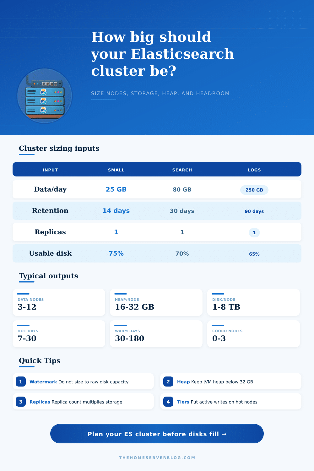
Building out a new Elasticsearch cluster is a hard task in tuning it to handle growth of data. Maybe you just want to store twenty gigs of logs per day and you’re off to the races. Soon enough, however, you’re thinking about node roles, watermarks, and how much memory you should gives to every node for its heap size.
When you plug in how much data you expect per day, and how long you want to keep things around, the calculator spits out those numbers for you. In other words, it prevents you from making a wild guess about how many variables to use based off your workload type.
How to Size Your Elasticsearch Cluster Correctly
By far most people get this wrong because they only think about available disk space, rather than usable space on a disk. You can’t count on having extra space for snapshots, shard relocation, or segment merging. If you max out a node, the cluster will stop accepting writes before it shows up on your dashboard. So it prompts you for what percent of the disk you’d like to use so there’s some headroom for that sort of thing.
It’s important to understand the difference between warm and hot tiers, which perform distinct tasks. Hot nodes serves the most recent queries and handle write pressure, so they should have plenty of CPU power and use fast SSDs. Warm nodes holds older data that’s still being searched but rarely changed. Mixing those kinds of workloads on the same hardware means that latency for searching compete with ingestion. By splitting those responsibilities in the calculator, you can see how many nodes you really need for each tier given your retention policy. For instance, you may believe that you need ten hot nodes, but the math reveal that moving older indices into warm storage asap would of let you get away with just three (and that’s where the savings happen).
The second common problem is heap memory. People are tempted to give Elasticsearch all the available RAM they have. But more than roughly thirty-two gigs isn’t good. The JVM will start wasting time using compressed object pointers above that number, which makes it less performant and costs you money. You never go over the heap size that keeps you running safely with queries and data volumes.
It factors in the number of replicas you have since those multiply (and even triple) your storage requirements. A lot of teams overlook this and then run out of disk when they routinely scale up. If you plan for replicas ahead of time, you avoid disk space problems during normal scaling operations.
The other way a cluster looks over-provisioned on paper (but still breaks) is with query concurrency. With fifty dashboards refreshing concurrently, it’s easy to saturate the search thread pools. That’s where coordinator nodes come into play, as they handle both parts of a query from the client side and traffic from clients, without hitting the data itself. Add coordinators according to the calculator when you’re reaching higher levels of concurrency than your data nodes can accommodate comfortabley. It’s a tiny architectural tweak that makes things more stable at scale. This is unnecessary in a quiet home lab scenario, but it is critical when your app is sending hundreds of requests per minute.
Similarly, details matter when it comes to intake rate. How much space do you need? That’s easy: raw log volume tells you how much space you need. What about CPU/network interface capacity? That depends on how fast the data arrives. Using an average doesn’t help you plan when your intake spikes in certain hours. To see whether your hot nodes can handle what you throw at them, you can enter the number of megabytes per second you expect. The tool then calculates whether they are up to the task by comparing with common benchmarks for various kinds of nodes. That way, you don’t end up with ample disk space but not enough processing power to keep up with logs coming in.
Nodes with master duties must be stable, don’t combine master duties with heavy data operations; that’s asking for trouble. Having 3 masters provide enough redundancy to handle elections without risking quorum problems if a node fails. The reference tables on the page show common configurations spanning lab use up through large log lake scale. This isn’t magic, these patterns are established after field testing in real world environments. Anything else typically means troubleshooting things that others who followed the pattern haven’t had to solve yet.
Finally, when it comes to sizing, you make tradeoffs: how much complexity do you want? How fast does it need to be? How much do you want to spend? If a constraint bothers you, buy more nodes. But at some level, the management overhead becomes greater then the benefit. With the calculator, you get a starting place according to today’s best practices. Where are your constraints? Where are your regions of excess capacity?
With this knowledge, you should size your first deployment correctly, then monitor how things actualy run. You’ll probably change as your data expands, but avoid the cycle of buying too many idle servers or too few struggling ones. Respect the heap limits, plan for usable space, and rely on tier separation to distribute the workload.