ETL Job Runtime Calculator
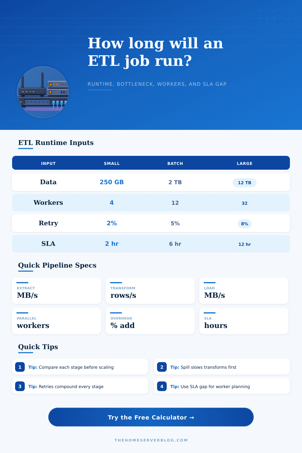
Estimate extract, transform, and load duration from data volume, throughput, workers, retry rate, network overhead, staging spill, and SLA target.
⚙Named ETL Presets
📊Pipeline Runtime Inputs
Runtime Results
🗂Current Pipeline Snapshot
📘Throughput Reference Table
| Pipeline type | Extract MB/s per worker | Transform rows/sec per worker | Load MB/s per worker |
|---|---|---|---|
| CSV files from NAS or SMB share | 25 to 80 | 15,000 to 60,000 | 20 to 60 |
| Parquet files from object storage | 90 to 250 | 60,000 to 220,000 | 60 to 180 |
| JDBC source to warehouse | 15 to 90 | 20,000 to 120,000 | 20 to 120 |
| CDC log replay or micro-batch | 10 to 70 | 10,000 to 80,000 | 15 to 90 |
| Compressed log archive restore | 40 to 140 | 25,000 to 100,000 | 35 to 110 |
🧮Stage Capacity by Configuration
| Configuration | Typical worker count | Best stage fit | Watch limit |
|---|---|---|---|
| Single VM cron job | 1 to 4 | Small extracts and direct loads | Memory and local disk spill |
| Airflow with task pool | 4 to 20 | Many independent table copies | Source connection throttles |
| Spark cluster | 8 to 200 | Large transforms and joins | Shuffle spill and skew |
| Warehouse ELT | Auto or slots | SQL transforms near data | Queue time and slot limits |
| Managed cloud ETL | 2 to 100 | Mixed jobs with retries | Startup time and partitions |
🔧Engine and Stage Comparison Grid
Extract
Transform
Load
Orchestration
📈Common Runtime Planning Sizes
| Project name | Data volume | Worker range | Planning target |
|---|---|---|---|
| Daily reporting mart refresh | 100 to 800 GB | 4 to 16 | Under 2 to 4 hours |
| Weekend warehouse backfill | 2 to 20 TB | 16 to 80 | Finish before business day |
| CRM import with dedupe | 20 to 250 GB | 2 to 8 | Protect source database |
| IoT partition compaction | 1 to 12 TB | 12 to 64 | Keep shuffle spill below 25% |
| Analytics log restore | 500 GB to 8 TB | 8 to 48 | Balance decompression and load |
💡Runtime Tuning Tips
The calculator transforms guesswork of running jobs into a concrete timeline for predicting outcome of any pipeline. It takes care of math behind it (for weekend backfills and nightly syncs), meaning you don’t need to wake up at 2am to see if your progress bar is still stalled. Instead, you know exactly when to expect your job to be finished, no more wondering if it will be done by sunrise, because your calculator gives a clear estimate based off the parameters you set.
When dealing with raw data volume, remember: gigabytes are not throughput. Instead, think in terms of effective throughput. The number of row and their structure will impact how they is compressed; a terabyte of Parquet files won’t behave like a terabyte of CSV logs.
Stop Guessing Your Data Job Times
Network overhead and retry rates add invisible drag that compounds over time, making extract stages look fast on paper but actualy slowing them down. You’ll see a three percent error rate as your source system keep dropping connections; the engine has to keep re-fetching chunks until it’s satisfied. This bloats runtime without adding any more rows so factor in those inefficiencies when estimating.
Most pipelines will grind to a halt at their transforms, and it’s almost always not because the transform itself require too much CPU, but because there isn’t enough memory. If a shuffle overflows into memory, the system will spill to disk, and that process should of slowed down your pipeline by orders of magnitude. The tool takes into account staging spill factor, so you can model what additional time you’re losing as your cluster reaches physical limit.
Adjust the number of worker to determine if you will improve things by adding more nodes. You can also see if you simply have idle capacity because bottleneck is I/O bound. Not all problems are solved by scaling up, and when it comes to jobs where the work is already network-saturated (e.g., extract), more workers will only get less and less value fast.
The most used part of load workflow is typically either batch commit interval size, increasing this decreases overhead dramatically, or tweaking partition sizes. This is especially true if small files are being ingested at high volumes, which is painful for warehouse loaders due to their per-write transaction cost. That’s why we let you model load throughput as a separate factor; it can help you determine if you’re struggling to transform data after it lands in the warehouse versus simply getting it there.
In an unpredictable world, service level agreements are rigid constraints. A 12 hour window for a big lakehouse compaction might sound reasonable except when accounting for maintenance windows and retry buffers. With the SLA gap metric, you’ll know precisely how many worker you must add (or how much more slack there is) to remain compliant. If it’s a negative, then congratulations, you’re already breaking your promise before you’ve begun the job. Use this to argue for infrastructure upgrades or to set realistic expectations with people who don’t yet grasp physics of data movement.
Baseline efficiency also varies by engine. Spark clusters are massively parallel, but they has to deal with startup time, which penalizes short jobs. For small data sets, a simple python script may seem faster due to its lack of distributed coordination costs. Dbt’s warehouse transformations differs from both managed cloud ETL services and native SQL procedures. Each have its own scaling profile. All of these affect the total duration. Choosing the correct engine, therefore, is a key part of proper planning.
This takes away all of the fear associated with the overnight run. If there are variables that can be planned for, plan for them. Stop looking at the logs and let the math do its thing. If you know the bottleneck is the join step, then optimize your joins before purchasing additional network bandwidth. If you know there’s a risk of spilling, then tweak your memory settings rather than blame slow disks for making things slow.
This way your data pipelines remains reliable, and the discussion changes from “why did my job fail” to “how can we scale this.