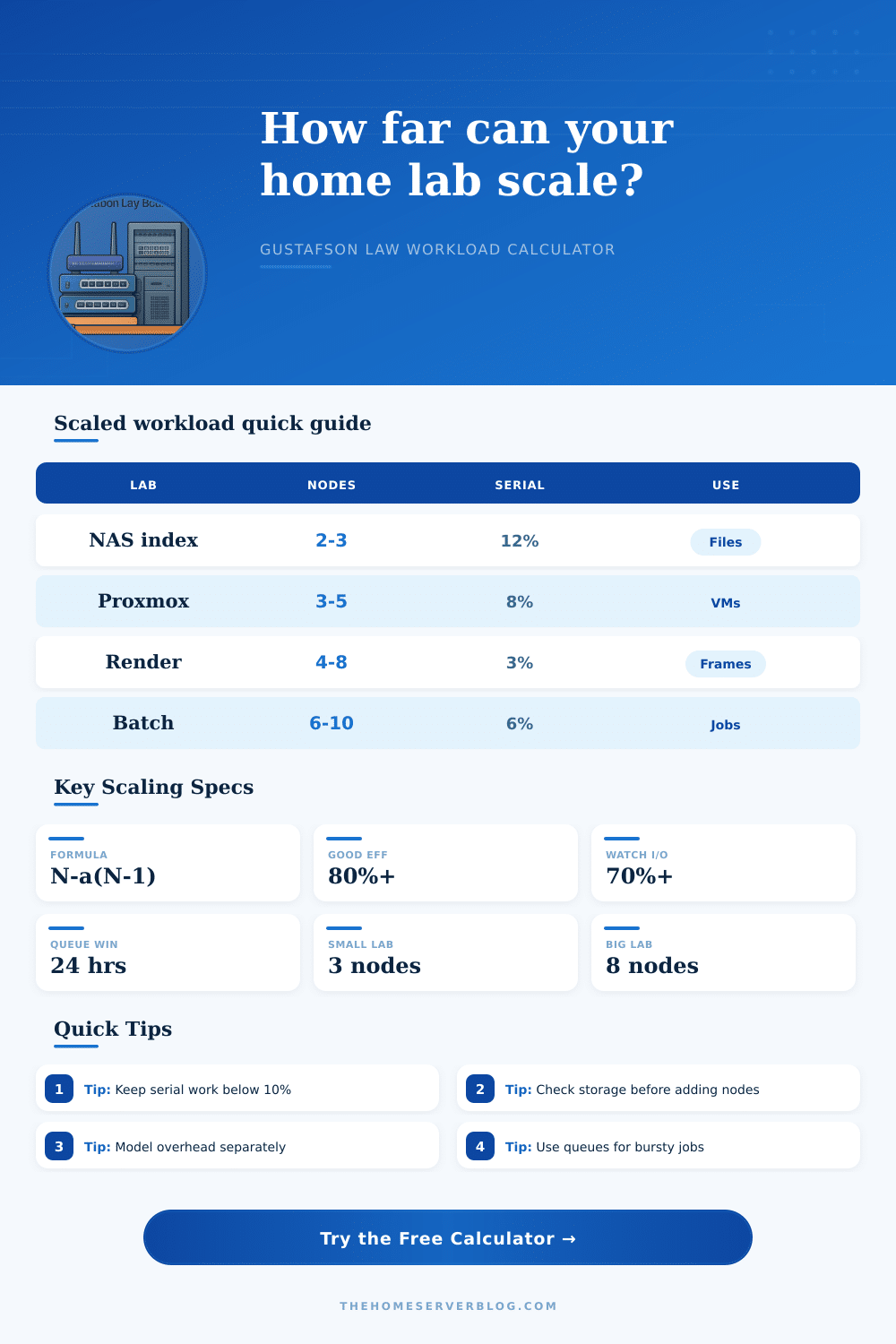
Gustafson Law Scalability Calculator
Estimate how much larger a fixed-time home lab workload can grow as you add render nodes, Proxmox workers, indexing hosts, or batch processors.
| Profile | Typical Serial Fraction | Dominant Shared Resource | Good Home Lab Signal |
|---|---|---|---|
| Proxmox worker pool | 6% to 12% | Scheduler, shared images, backup target | Jobs start quickly and VM locks are rare |
| Render node frame farm | 2% to 6% | Asset reads and result writes | Nodes spend most time rendering frames |
| NAS metadata indexing | 10% to 20% | File walks, catalog updates, small I/O | Index commits do not stall scans |
| Nightly batch processing | 4% to 10% | Queue broker and database writes | Queue drains before the maintenance window ends |
| Media transcode lane | 3% to 9% | Source reads, destination writes, hardware encoders | Workers are CPU or encoder limited, not share limited |
| Nodes | 3% Serial | 8% Serial | 15% Serial | Interpretation |
|---|---|---|---|---|
| 2 | 1.97x | 1.92x | 1.85x | Nearly linear for most home jobs |
| 4 | 3.91x | 3.76x | 3.55x | Small cluster sweet spot |
| 8 | 7.79x | 7.44x | 6.95x | Shared storage starts to matter |
| 12 | 11.67x | 11.12x | 10.35x | Coordination needs measurement |
| Fabric Or Storage Path | Practical Sustained Ceiling | Useful For | Scaling Note |
|---|---|---|---|
| 1 GbE SMB/NFS | 90 to 115 MB/s | Light indexing, backup checks | Two workers can saturate it quickly |
| 2.5 GbE home switch | 230 to 285 MB/s | Small render cache, media queues | Good match for 3 to 5 modest nodes |
| 10 GbE direct or switch | 850 to 1150 MB/s | Render assets, VM image farms | Often enough for 6 to 10 workers |
| Single SATA SSD pool | 350 to 520 MB/s | Scratch queues, staging data | Random I/O may matter more than MB/s |
| NVMe mirror or stripe | 1800 to 5500 MB/s | Heavy temporary datasets | Network can become the new ceiling |
| Project | Fixed Window | Best Scaling Lever | Warning Sign |
|---|---|---|---|
| Nightly Proxmox maintenance tasks | 6 to 12 hours | Separate queues by storage target | VM locks and backup target spikes |
| Weekend render batch | 24 to 48 hours | Keep assets local or cached | Many idle nodes waiting for scene files |
| Fresh NAS photo index | 8 to 36 hours | Shard directories and merge metadata late | Catalog writes dominate scan time |
| Media library transcode burst | 12 to 72 hours | Balance encoders and disk writes | All workers writing to one slow pool |
Few larger nodes
Best when software has a meaningful serial phase or each job needs high memory locality.
Good for indexingMany small workers
Best when tasks are independent, short, and easy to queue without shared write contention.
Good for framesHybrid pool
Best when a coordinator, fast cache, and several worker nodes can split the workflow cleanly.
Good for ProxmoxTwo old servers + more compute power = your starting point. You might add a third node to render on weekends or back up Proxmox at night because you think it will go faster. You can expect linear performance gain. Ouch. Now you hit the wall. Nodes waits for locks on shared storage. Alternatively, the catalog merge step take longer regardless of how many cores sit idle, which causes the finish time to suffer.
Enter Gustafson’s Law. While Amdahl’s Law looks at how fast you can make a fixed problem, Gustafson proposes that if you throw in more hardware, you can work on a bigger problem in the same period of time. That makes sense for someone with home lab, especially when you have only so much time. It changes the question from “how fast” to “what do I get?” How many more frames can I push through until Sunday night?
How to Scale Your Home Lab Correctly
This page has a calculator showing this tradeoff where you can specify a serial fraction and then watch the workload volume increase as you scale up to n+1 nodes. In all scaling stories, primary limitation is your serial fraction, which is defined as the fraction of your workflow that can’t be parallelized. That includes splitting up jobs for distribution and merging them back together in an archive file. It also includes writing the final report to a single database or even just starting up the job queue in the first place. Adding 50 nodes won’t get rid of that bottleneck entirely if it’s only 10% of your process. It’s still there.
By applying your estimated serial percentage to your number of nodes (plus overhead buffer), tool shows that constraint for you. More often than not, the serialization isn’t due to CPU logic but hidden somewhere else… Like storage access. Maybe you’ve got eight beefy threads waiting on one SATA drive to spit out some metadata, turning your parallel compute into a serial traffic jam.
Knowing about that I/O dependency is worth more then a whole other graphics card. Before the processor’s going to hit its limit, the performance will be capped by storage bandwidth instead. Even a basic one-gigabit ethernet link can sustain only about ninety megabytes of traffic per second, quickly overwhelmed if three nodes is trying to load large asset libraries all at once. The reference tables provided with the calculator spell out these achievable bandwidths for typical home networks, so that you’ll know why what would of been a nice speedup on paper just isn’t happening in reality.
If you expect adding more workers to process more data, but your increased data rate exceeds what your network can handle, then the extra heat from those additional compute units isn’t worth it. Make sure that the number of workers matches size of the data pipe. Getting a ten-gigabit or two-and-a-half-gigabit network is often a better step towards improved real-world scaling than getting an additional low-end worker node.
This includes everything from the cluster config. What do you do differently? Embarrassingly parallel workloads like rendering frames, where each frame is an independent image… Have very low serial fractions at around two to three percent. Sweeping a giant NAS library with file system walking and lots of catalog contention adds significant overhead. This cause higher serial estimates on storage sweeps than equivalent passes on backup verification tasks or media transcoding jobs. The calculator’s built-in presets are aware of this and adjust the I/O profiles and coordination pressure of each workload type to match.
Fitting a database indexing job into a render node profile will result in overly optimistic results that never materialize in practice. It’s a method of making yourself honest about your limitations in infrastructure. When the math says your bottleneck is storage or your coordination point is slow, you can’t bury your head and pretend your cores makes all the difference. Instead, you realize some part of your workflow will always be serial; and from there, you optimize for throughput given your real-world constraints instead of pursuing the elusive promise of perfect efficiency.
Whether you’re working with a tiny backup verification pool or a bigger mixed homelab burst environment, knowing what you can do eliminates the frustration. It’s less about going fast forever, and more about getting a solid volume done reliably. The original fantasy of infinite processing power returns, but this time, with an accurat map to where the road really stops and how to construct around it.