IPv6 Solicited Node Multicast Calculator
Derive the solicited-node multicast group, Ethernet multicast MAC, and Neighbor Discovery load for a home lab IPv6 segment.
⚙Home Lab Presets
🔧Multicast Inputs
Calculation Breakdown
🖧Equipment and Network Spec Comparison
📘Solicited-Node Derivation Reference
| Step | Value Used | Formula | Home Lab Meaning |
|---|---|---|---|
| Input address | Unicast or anycast IPv6 | Use full 128-bit address | Applies to global, ULA, and link-local addresses. |
| Low 24 bits | Final 6 hex digits | Address AND 0xFFFFFF | Hosts with the same low 24 bits share a solicited-node group. |
| IPv6 multicast | ff02::1:ffXX:XXXX | Append low 24 bits | Neighbor Solicitation packets target this link-local group. |
| Ethernet MAC | 33:33:ff:XX:XX:XX | Map IPv6 multicast to MAC | Switches see this as a Layer 2 multicast destination. |
📡NDP Behavior Table
| Traffic Type | Packet | Default Count | Where It Matters |
|---|---|---|---|
| Duplicate Address Detection | Neighbor Solicitation | 1 transmit | When a host brings an IPv6 address up on an interface. |
| Neighbor resolution | Neighbor Solicitation | Up to 3 tries | When a node needs the Layer 2 address of another IPv6 node. |
| Neighbor response | Neighbor Advertisement | As needed | Sent back by the target node, usually unicast after resolution. |
| Switch filtering | MLD report | Per group | Lets a snooping switch avoid flooding all IPv6 multicast frames. |
📊Common Home Lab IPv6 Sizes
| Scenario | Typical Nodes | Address Pattern | Multicast Watch Point |
|---|---|---|---|
| Small server VLAN | 5 to 15 | Static ULA plus link-local | Usually light unless each service has many VIPs. |
| Proxmox or lab cluster | 3 to 10 | Host, bridge, VM, and container addresses | Count guest addresses, not just physical hosts. |
| IoT VLAN | 25 to 150 | Mostly SLAAC or DHCPv6 | Low-end Wi-Fi bridges may flood multicast more often. |
| Privacy-client WLAN | 10 to 80 | Temporary privacy addresses | Address churn increases DAD and group membership changes. |
🧮Standards and Practical Limits
| Reference | Value | Used By Calculator | Practical Note |
|---|---|---|---|
| IPv6 multicast scope | ff02 link-local | Solicited-node group prefix | Traffic stays on the local link and does not route between VLANs. |
| Solicited-node suffix | 24 low-order bits | Group and MAC derivation | The same suffix can be shared by more than one IPv6 address. |
| Ethernet multicast prefix | 33:33 | Layer 2 destination MAC | Only the low 32 bits of IPv6 multicast map into Ethernet. |
| SLAAC subnet size | /64 | Prefix warnings | Use /64 for normal LANs unless you know the exception. |
💡Calculation Tips
Plug in a new server to your home lab switch, wait for it to come online, and then observe your network capture tool with a flurry of multicast traffic that appears suspiciously like a denial of service. Not an attack. This is IPv6 doing precisely what it’s designed to do.
The source of confusion usually relates to address resolution within IPv6. Whereas IPv4 employs broadcasting to all device on a subnet, IPv6 employ multicast groups (called solicited-node addresses). Each device join these groups so that it can listen for neighbor discovery packets. How much traffic is generated here depend upon how many addresses are in use as well as how frequently each one need to verify its identity on the link.
How IPv6 Multicast Works
To make life easier, the calculator above handle the math for you by taking your subnet details and projecting the resulting load. Just feed in what you know about the subnet, such as the IP version, the IPv6 address, the prefix length, the number of nodes on your VLAN, and how many addresses each one has. It then calculate the relevant Ethernet MAC address and multicast group. It also calculates how many probes you’ll see while resolving neighbors and starting up. That way, if there’s a problem with delay, or you want to adjust switch settings based off this, you’ve got some concrete numbers to work with instead of more vague workings of the protocol.
To get a more realistic view it’s important to understand what goes into your calculations. For example, the stability of the address matter (a laptop with privacy enabled vs a stable server). Why? Because moddern operating systems change their temporary address all the time. That means every single new address has to trigger a neighbour solicitation and duplicate address detection.
You will have dozens of virtual interface if you use a hypervisor like Proxmox or run a Kubernetes cluster, which in turn produce dozens of different traffic streams. You can adjust the number of addresses and nodes via the calculator. Otherwise you’ll grossly underestimate how many packets are actualy flowing.
So what does it give you? In my case, I got the following:
That’s the group for the node I’m asking for. Every multicast group begins with ff02::1:ff followed by the remaining 24-bits of your own unicast address. So two different unicast nodes that have same last six hex digits will both belong to the same multicast group. It is a pretty clever way to keep things manageable as an address space. But this also causes some traffic to collide where you might not expect it.
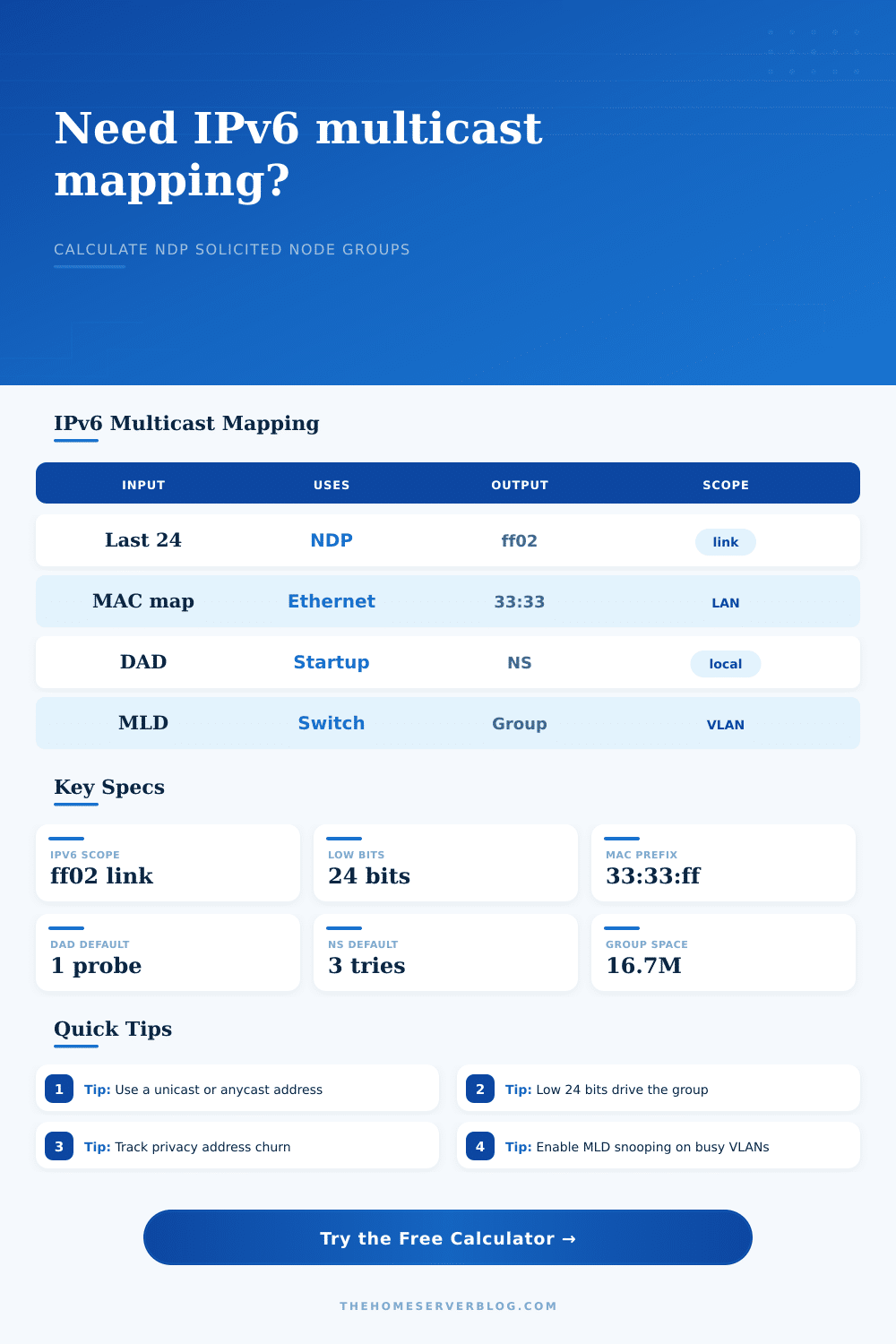
You’ll see the remaining bits in the multicast group used to create your Ethernet MAC address, mapping back to prefix 33:33:ff. Those are the bits that your switches uses to forward frames on. If multicast listener discovery snooping is not turned on, all ports within the VLAN that can listen to multicast traffic will recieve every multicast packet. That is the problem folks get wrong; they blame their lack of bandwidth, when the actual problem is they’re just having multicast frames flooded to them inefficiently.
A second important metric is probe volume. This is the number of solicitation packets sent out for neighbor discovery (to learn a device’s layer 2 address) and duplicate address detection (to confirm that an address hasn’t been used already). By default, it assume a reasonable amount of retries according to typical policies. You can set a stricter or leaner policy, which means more or fewer packets but higher or lower reliability. For example, if your IoT VLAN is densely populated with devices that may come online and offline frequently, you’ll likely see some greater retry counts. That way you can determine if you want to tweak your switch aging timers, or turn on more aggressive snooping instead.
On the page are the reference tables laying out the derivation steps and common scenarios. You can see how it’s deterministic. How the group is formed isn’t random.
The question becomes: how do you manage the total load when there are hundreds of devices? Client-side privacy extensions result in a churning effect: old addresses expire; new ones appear. This creates a small burst of traffic each transition, add it all up over time and it starts to become significant. The calculator helps you visualize that cumulative effect.
So in conclusion, no, IPv6 multicast isn’t a bug. It’s a feature and it needs to be made visible. With addresses mapped back to their multicast group, you have control over what is happening at layer 2. Tuning your switches to filter well help prevent the hidden cost of flooding traffic you didn’t want in the first place. And ultimately, we want an efficient and quiet network where discovery occurs without disturbing production traffic. That starts with clarity. Understanding how solicited-node works will help bring that clarity. You build the network, but the protocol creates the noise.