Kruskal Minimum Spanning Tree Calculator
Sort weighted graph edges, run union-find cycle checks, show selected and rejected edges, and detect when a sparse graph becomes a minimum spanning forest instead of a single MST.
| Sorted Rank | Edge | Weight | Input Order | Cycle Check |
|---|---|---|---|---|
| 1 | A-B | 0 | Paste edges | Waiting |
| Step | Edge | Roots Before | Action | Component Count |
|---|---|---|---|---|
| 1 | A-B | A / B | Run Kruskal | 0 |
| Component | Vertices | Selected Edges | Component Weight | Status |
|---|---|---|---|---|
| 1 | A, B | 0 | 0 | Waiting |
| Kruskal Concept | What This Calculator Shows | Why It Matters | Common Home Lab Analogy |
|---|---|---|---|
| Sorted edge list | Every valid edge ranked by weight | The lightest safe edge is considered first | Cheapest latency or shortest patch first |
| Union-find roots | Root pair before each edge decision | Different roots mean no cycle yet | Two islands can be linked safely |
| Cycle rejection | Same-root edges marked rejected | Cycles add weight without connecting more vertices | Redundant loop blocked by design |
| Minimum forest | Multiple components after all edges | Sparse or disconnected graphs lack a full MST | Unpatched rack group stays isolated |
Imagine you have a mess of cables and a set of switches. Your goal is clear: hook everything up as cheap as possible. On paper, it sounds easy enough. But in real life, it gets gnarly when you consider that the lowest-cost cable might create a loop, which ruins your switching strategy. How do you select the single best connection without inadvertantly completing a circuit?
Here comes Kruskal’s algorithm: It removes the guessing game by listing all possibilities from least-expensive to most-expensive and selecting each connection until no cycles is left. That is the main idea. It sounds very simple. But let me give an example. Think of islands, connected by other bridges, at different prices. How do we connect all those islands with minimal spending?
Understanding Kruskal’s Algorithm
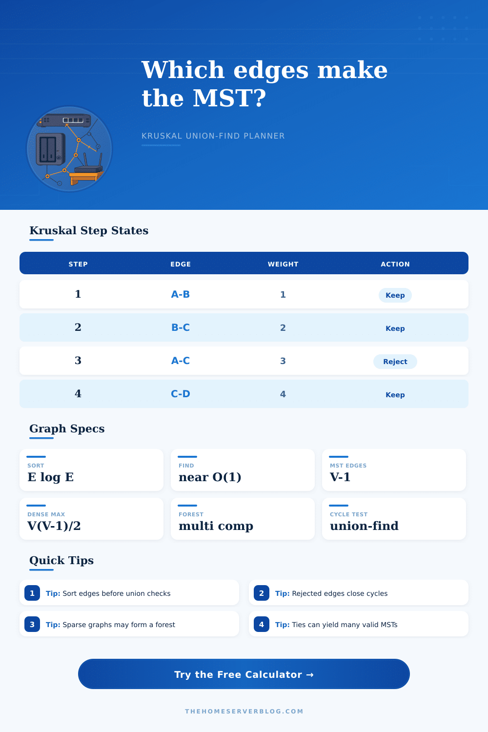
Well, you begin with lowest priced bridge. And if there is another land mass on each side then you add it. If not (i.e., it would form a loop) you ignore it. Continue until all of the islands can be reached. That’s what the calculator does. It figures out for you that it doesn’t need to find the base of the bridges in your head, but rather just sort through them. It also detects cycles to prevent building loops.
The tie breaking is where most fall down. And this happens because there are multiple edges with the same weight. Tie them together, and cost is the same either way. But what about the topology? That’s different now. Maybe two cables runs parallel to each other. Both are the same cost, but only one goes over the ceiling. Physical constraints matter for installs. The tool lets you define how it handles ties between edges with the same weight: Should it be based off input order? Or should it sort the endpoints alphabetically? This is a very small detail that often sets the theoretical model apart from an actual install plan.
Knowing about density will also help you read what they spit out. For a sparse graph, there are few edges relative to its nodes. If you feed it a disconnected network, it won’t just fail silently; it will tell you it found a minimum spanning forest. That means it’s a set of trees, one per island of isolation points, with an optimum path for every tree but not necessarily across all trees. It is important to understand the difference between a single MST and a set of forests. A single MST suggests everything is connected, while a set of forests tells you some things aren’t. The output tables neatly lay out pieces so you can quickly see exactly how the graph fails.
How? A lot of that is done by the union-find method under the hood: it groups nodes into sets, then asks whether two vertices are already part of same set before adding that edge. If so, it doesn’t create a cycle. Otherwise, you could link A to B but they’re already linked by C and D, and that unecessary wire creates latency and costs money while not helping your reachability. The step-by-step grid in the tool shows those decisions being made in real time. It shows which edges is joining previously separate sets and which are getting tossed because they close a loop.
In reality, networks don’t look like textbook cases. While physical cabling is unlikely to include negative numbers, abstract optimization problems often do. The algorithm doesn’t know if a number is positive or negative, just which one is smaller. If the number links previously unconnected parts of the network, it will always pick that one. That makes this approach broadly applicable. Routing power lines? Fiber optics? Either way, greedy selection with cycle avoidance is the same idea.
Ties and sparse inputs require extra attention If you are highly connected, then lots of your edges will be pruned out as redundant. It’s not an error; it’s the nature of the beast. Lots of rejections, but don’t think of these as errors. Think of them more like pruning. You get the minimal backbone. The graph enforces a tree structure, which means it must prune any excess. By definition, there can be no loops in a tree. Each rejected edge is a path that was either too expensive relative to others, or it formed a loop with other ones already included.
So what’s the real value here? Visualisation. It takes something as abstract as networking and makes it concrete. You’ve got the decision trail, you’ve got the sorted list. You can use tie-breaking to pick the best edges when costs are equal for safety reasons. You see where there might be a missing link between two subnets based on the input data. It takes the mystique out of network design, breaks it into logical, separate steps. It makes sense of the chaos while keeping cost and connectivity front and center.
So, it is about efficiency. Testing every conceivable set of cabling combinations isn’t necessary. It would of been mentally exhausting, and it would take too long on the computer. If you sort first and then check for cycles, you can solve this in linear-logarithmic time (relative to number of edges). It goes quick, it’s trustworthy, and you know how it works. You get a simple, uncluttered structure that ties together everything that matters without wasting resources by runninging in circles.