Prim Algorithm Minimum Spanning Tree Calculator
Plan how Prim's algorithm will execute on an undirected weighted graph before you run it in a network lab, topology simulator, or graph service.
| Choice | Best graph shape | Memory pattern | Prim operation profile |
|---|---|---|---|
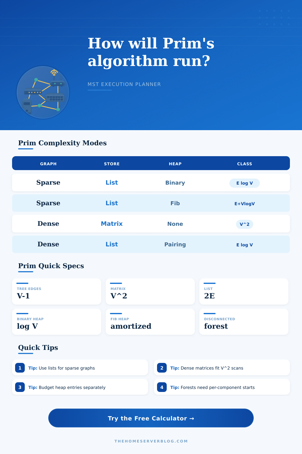
| Adjacency list + binary heap | Sparse LAN, WAN, route maps | Stores 2E weighted arcs plus heap | O(E log V), predictable and common in production code |
| Adjacency list + Fibonacci heap | Large sparse graphs with many decrease-key calls | Higher pointer overhead than binary heap | O(E + V log V), strong theory, heavier constants |
| Adjacency list + pairing heap | Sparse or medium-density lab graphs | Pointer heap with practical decrease-key behavior | Often close to Fibonacci behavior without full complexity |
| Adjacency matrix + scan | Dense complete or near-complete test matrices | V² weights even when edges are absent | O(V²), no priority queue pressure |
| Implementation | Extract-min | Decrease-key | Total Prim class |
|---|---|---|---|
| Array or matrix scan | O(V) | O(1) | O(V²) with adjacency matrix |
| Binary heap | O(log V) | O(log V) | O(E log V) using adjacency lists |
| Fibonacci heap | O(log V) amortized | O(1) amortized | O(E + V log V) using adjacency lists |
| Pairing heap | Amortized logarithmic | Very low amortized in practice | Usually modeled between binary and Fibonacci |
| Density band | Edge count guide | Suggested representation | Why it matters |
|---|---|---|---|
| Tree-like | E about V - 1 | Adjacency list or CSR | Matrix cells mostly empty; heap stays small |
| Sparse network | E below 5V | Adjacency list + binary heap | Good balance for routed and switched topologies |
| Medium mesh | E from 5V to 0.25V² | List, CSR, or pairing heap | Heap pressure grows; buffer becomes important |
| Dense graph | E near V(V-1)/2 | Matrix scan | O(V²) scan can beat heap overhead |
| Output | Formula used | Notes | Planning use |
|---|---|---|---|
| Tree or forest edges | V - components | Prim returns a forest if the graph is disconnected | Checks whether enough edges exist to connect each component |
| Matrix memory | V² × bytes per weight | Includes absent edge slots | Useful for dense lab matrices and classroom demos |
| List memory | 2E × arc bytes + arrays | Undirected edges store two directed arcs | Best for most home lab and WAN graphs |
| Step playback time | scaled steps / steps per second | Shows animation time, not CPU benchmark time | Keeps visual demos from becoming too slow |
This is the kind of messy, interconnected network diagram with which you’re tasked: Find the cheapest way to connect every node without creating loops. (Sounds familiar?) (Sounds familiar?) You need a minimum spanning tree solution, and one such method is Prim’s algorithm, which begins with a starting point and adds the next-cheapest option along each step outwards until everything are connected. Sounds straightforward, except that how the growth happens depends off your choice of priority queue (how do you keep track of options?) and storage mechanism (what does data look like?). Before running simulations or writing any code, you need to plan ahead.
If you know how dense your network is (edge density) and how many nodes you have, you can just plug that into the calculator and let it do the work. No need to guess at your memory estimate or coefficients. Everyone thinks an adjacency list is better because it’s smaller than a matrix. That’s true if your network is sparse. A region fiber ring are sparse. Most of the switches don’t talk to each other on a typical office LAN. In those kinds of graphs, you have lots of vertices and few edges. So keeping just the existing connections are enough to keep your memory footprint small and perform heap operations within reason.
Plan Your Data Structures
That’s all good, but then again, what happens if you is working with a very connected graph, like a complete mesh test case, or an interconnection fabric spanning a whole data center? In that case, where each node have almost direct connections to nearly every other one, the prior hunch turns upside-down: managing the heap structure and pointers could of being too slow, while a simple array may be much faster then just scan. If it’s near-full, the time to do a binary search on a long list would cost more than just doing a linear scan.
You can switch between the two to see at which point the crossover occur for your own datasets. And it estimates how many operations will occur, so you can figure out whether E log V might really be cheaper then V squared in your cases. How you store your graph matters too but so does type of priority queue. You might choose something like a binary heap, and why wouldn’t you? Then you can get guaranteed logarithmic time to get the min-distance node and update its edges, which is pretty good. They’re simple to code they work well.
From a theoretical standpoint, Fibonacci heaps has an amortized benefit when performing decrease-key operations, but they’re complicated beasts with a lot of pointer juggling, which makes them more memory intensive than the other two and with some very high constants in practice. For all but the largest of graphs, the real world isn’t that big. Even a pairing heap will perform better in reality for most real-world networks, even though it technically has a worse complexity class because the code simply executes faster.
Also, what about disconnected components? A network with isolated segments means that Prim’s algorithm will only visit one such segment beginning at your root node. So what happens? You get a spanning forest instead of a spanning tree! You can indicate the amount of components you have, which then updates the memory requirements (and expected edge count) on the calculator. For simulation, this is an important step to plan ahead; otherwise you’re going to allocate memory for connectivity that doesn’t even exist in your topology.
For example, it can help budget memory. Memory budgeting is also easy to get wrong quickly and hard to fix later. When you’re working with large matrices (like V squared) in floating point numbers, the size of your matrix representation matters (e.g., 64-bit float vs. This is a 32-bit integer. The tool calculates what this means in terms of RAM usage and provides a buffer. This helps you avoid out-of-memory crashes while doing batch processing or visualizations. It makes concrete moments (milliseconds, megabytes) out of abstract complexity theory.
In the end it’s all about choice and growth. Start small, grow slowly, only take the cheapest thing you can afford. Each step of that growth should be done as efficient as possible. Otherwise, it becomes a bottleneck. That’s why getting the data structures correct is important. Ultimately, connecting the dots is only half the battle; you also don’t want to exhaust your systems while doing it. Just like untying a bird’s nest, you need the right tools and a good plan before you start.