Database materialized view planning
Materialized View Size Calculator
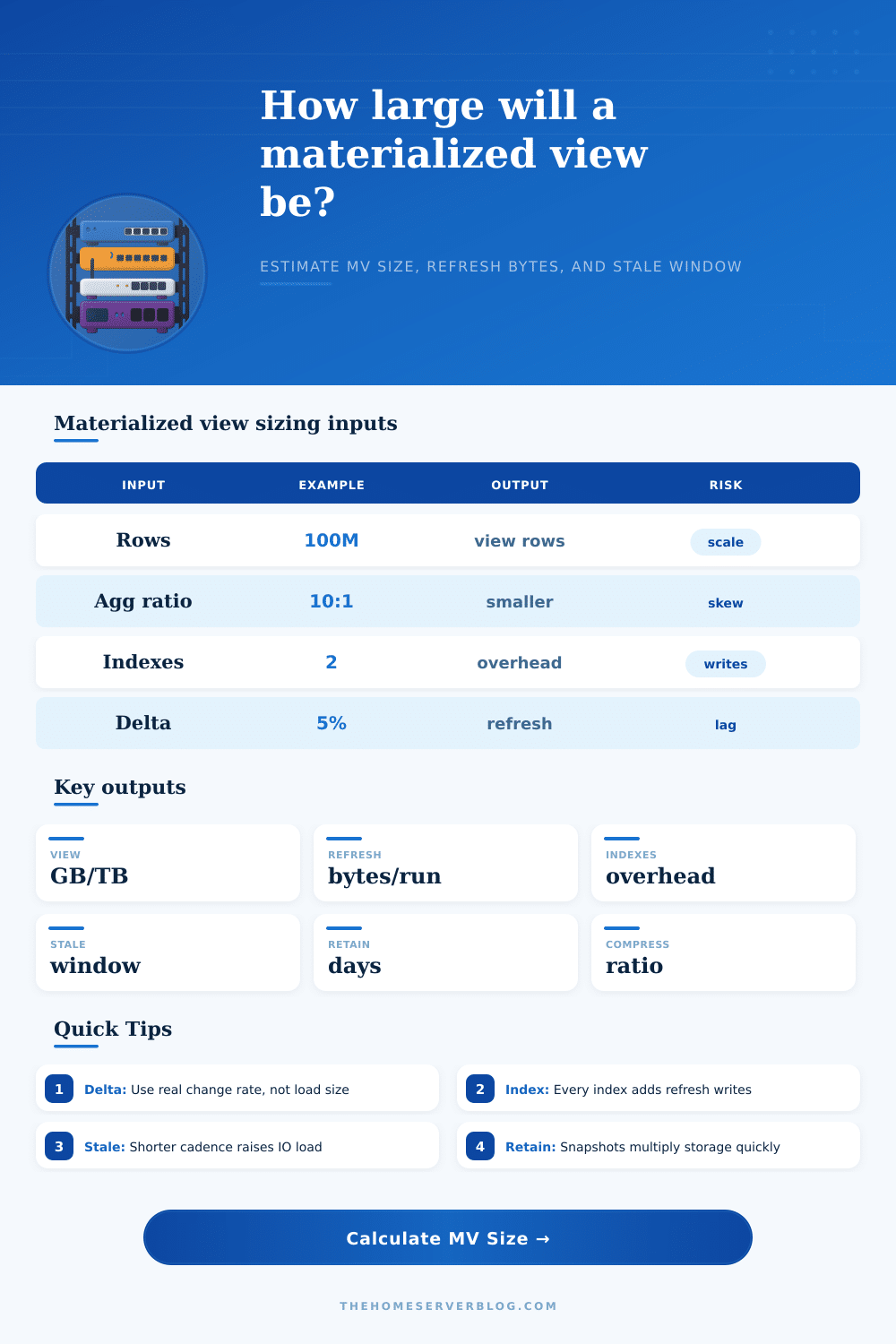
Estimate materialized view storage, refresh bytes per run, index overhead, retained snapshot size, compression impact, and stale data window from source rows, column width, aggregation ratio, change rate, and refresh cadence.
Storage breakdown
Refresh workload
| Component | Formula | Rows or runs | Size | Planning note |
|---|---|---|---|---|
| View table | MV rows x row width | 0 | 0 MB | Calculated after inputs load |
Rollup MV
High aggregation ratio, moderate row width, and small indexes. Best for dashboards that query repeated grouped metrics.
Snapshot MV
Aggregation ratio near 1:1. Storage follows source scale, so compression and retention days become the major factors.
Incremental MV
Refresh bytes depend on delta percentage and index count. Good when change sets are much smaller than the full source.
Concurrent MV
Lower read blocking, but peak footprint can approach an extra full copy during rebuild and swap operations.
| Strategy | Best fit | Refresh bytes | Peak storage | Stale window |
|---|---|---|---|---|
| Complete refresh | Small MVs, nightly reports, simple rebuilds | Full MV table plus indexes every run | Usually one to two active copies | Refresh interval plus rebuild time |
| Incremental refresh | Low delta fact tables with change logs | Changed rows plus affected aggregates and indexes | Active MV plus delta staging | Refresh interval plus apply time |
| Concurrent rebuild | Read-heavy dashboards requiring availability | Often similar to complete refresh | Can temporarily double the active footprint | Old view visible until swap completes |
| Partition refresh | Date-partitioned facts and rolling windows | Only changed partitions plus indexes | Active MV plus refreshed partitions | Partition cadence and publish schedule |
| Streaming aggregate | Operational metrics and near-real-time needs | Small frequent writes with higher maintenance overhead | Active MV plus state store | Seconds to minutes when tuned well |
| On-demand refresh | Ad hoc reports and low-use summaries | Only when requested or scheduled manually | Depends on rebuild method | Unbounded until someone refreshes |
| MV pattern | Typical ratio | Row width behavior | Index choice | Storage warning |
|---|---|---|---|---|
| Daily metric rollup | 100:1 to 10,000:1 | Few dimensions, numeric measures | Date and dimension keys | Usually compact unless many dimensions are retained |
| Customer summary | 10:1 to 1,000:1 | Wide profile columns and counters | Customer key plus segment filters | Wide rows can offset strong aggregation |
| Facet count table | 1,000:1 or higher | Small keys and counts | Facet value and category | High cardinality facets can expand quickly |
| Current snapshot | 1:1 to 5:1 | Similar to source projection | Lookup keys and freshness columns | Retention multiplies storage almost linearly |
| Time bucket MV | 10:1 to 100,000:1 | Bucket keys plus aggregate measures | Time, tenant, and metric keys | Short buckets and many tenants lower the ratio |
| Join acceleration MV | 1:1 to 50:1 | Often wider than source fact rows | Join keys and filter columns | Denormalized text columns can dominate size |
Speed: If you’re running a reporting dashboard that queries frequently, then materialized views will make your queries fast! But there is cost for this speed. Data freshness means your results may be stale. Refresh overhead means you pay compute resources to refresh the view.
You will need to store result somewhere, though most engineers think this won’t matter since their source tables aren’t that big. Most engineers think “oh my source table isn’t very big, I’ll use the free storage”… But when things gets busy in production, numbers add up quickly and you hit capacity. There’s no magic number that solves all problems; instead, knowing how each input translates into your infrastructure matter more than anything else.
The Hidden Cost of Speed
First, think about aggregation ratio. How many source rows is being aggregated down? And think about nature of those rows, for example, do you have one billion transaction rows that get summed up as daily totals for each customer? That’s a good start; you’ve reduced the row count by 100:1. But now look at size of the rows you’re keeping: For each customer, how much wider does the row become with all its columns? (If there are any text fields or JSON blobs, the answer may be: pretty darn wide.) Remember, a wide denormalized view isn’t going to use fewer bytes than three narrow view.
What does your schema design store and measure? More indexes improve query performance, at the cost of more bloat. Indexes speed up access to the materialized view, so far so good. But now every time it is refreshed, indexes need updating too. More indexes make refresh slower because each one adds write amplification. A larger set of indexes also takes up more disk space, which is proportional to their row count and key width.
If you incrementally refresh infrequently-changing data, then fine. Otherwise, the refresh may swamp your IOPS budget, especially if your dataset change often and has many indexes. Different strategies pay differing penalties for read speed vs. Write cost; see this table of references for details. Convenience comes at price of extra overhead in maintaining the indexes.
The stale window is how long data remains out of date before it is refreshed again. Five minutes seems responsive. However, it increases number of daily refreshes by 12x over an hourly schedule. That’s 12x more index updates and 12x more transaction log pressure. If you run concurrent rebuilds with a shadow copy while swapping, then it could be doubling your maximum storage footprint.
Unfortunately most teams set their timing based off user expectation not infrastructure capacity. When everyone logs into the same dashboard, things tend to slow down. These problems is lessened through compression, but not entirely. Fields like encrypted values or short text strings aren’t well suited to columnar compression. High cardinality numeric fields are.
When in doubt, don’t assume a 40% reduction across every column (you’ll likely be undersizing your storage by a wide margin when reality hit). Compound this mistake through retention policies. These are typically set to keep the last seven days worth of snapshots for troubleshooting purposes, which then multiplies your active footprint by a factor of seven. Add in regular refreshes and uncompressed indexes, and suddenly the overall cost will shock even veteran engineers.
That doesn’t mean we’re looking to shrink everything for its own sake, rather it means making storage choices that match kinds of queries people run. Running a slower complete refresh overnight can save a lot of I/O during the day if nobody runs the view after-hours. Offering a near-realtime version requires more disk but less lag if your users want it. This isn’t a free-lunch situation; there’s just a set of tradeoffs between storage, speed and freshness.
But before you roll out your next materialized view, take twenty minutes to figure out what it’s realy going to cost you with these tools. Be honest about your delta rates. Add up all the indexes you’re going to need. Factor in compression based off column types. Run the numbers ahead of time rather than troubleshooting storage warnings at 2 AM after the bill drops and no one can recieve notice who approved that last refresh job.