Nutanix Erasure Coding Calculator
Model EC-X style data/parity strips, RF2 or RF3 baseline capacity, cold data eligibility, usable capacity, savings, and rebuild read impact for Nutanix home lab and edge clusters.
The calculator estimates logical usable capacity after reserving raw space, then blends normal RF consumption for hot data with EC-X consumption for cold data. It is a planning estimate, not an AOS guarantee.
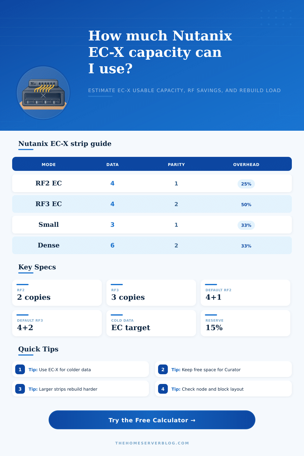
| EC-X style | Availability target | Storage multiplier | Best use |
|---|---|---|---|
| 3+1 | RF2-like, one missing fragment | 1.33x raw per logical TiB | Small clusters where a 4+1 strip does not fit well |
| 4+1 | RF2-like, common default planning case | 1.25x raw per logical TiB | General cold VM, files, object, and archive data |
| 4+2 | RF3-like, two missing fragments | 1.50x raw per logical TiB | Higher resilience clusters with enough nodes and blocks |
| 6+2 | RF3-like with lower percentage overhead | 1.33x raw per logical TiB | Large capacity clusters; watch rebuild and locality cost |
| Cluster profile | Typical RF | Cold data target | EC-X note |
|---|---|---|---|
| Home lab VM mix | RF2 | 40% to 65% | Useful when templates, ISOs, and idle VM data dominate |
| Nutanix Files or Objects | RF2 or RF3 | 65% to 90% | Often a strong EC-X fit because much data is read cold |
| VDI or active database | RF2 or RF3 | 10% to 35% | Frequent overwrites reduce EC-X benefit and may add decode cost |
| Backup and archive target | RF2 | 75% to 95% | Large sequential cold data usually gives the clearest savings |
| Planning check | Why it matters | Good signal | Risk signal |
|---|---|---|---|
| Nodes vs strip width | Data and parity fragments should spread across failure domains | Nodes exceed data plus parity | Strip width equals or exceeds nodes |
| Blocks or chassis | Block awareness improves placement when enough domains exist | Several blocks for capacity clusters | Single-block clusters |
| Free capacity | Curator needs room while data transitions from RF to EC-X | 15% or more reserved | Very full containers |
| Working set | Hot data remains more RF-like while cold data benefits most | Low overwrite, low working set | High churn or heavy random writes |
| Example | Raw cluster | EC-X plan | Expected result |
|---|---|---|---|
| 6-node files share | 288 TiB raw | RF2, 4+1, 75% cold | Roughly 40% more usable than RF2 only |
| 8-node VM cluster | 384 TiB raw | RF2, 4+1, 55% cold | Good capacity lift with moderate decode exposure |
| 12-node RF3 apps | 576 TiB raw | RF3, 4+2, 50% cold | Large gain versus three full RF copies |
| Backup target | 768 TiB raw | RF2, 6+2, 90% cold | High savings; validate rebuild window carefully |
With erasure coding, you start out with what seems like a big enough cluster: a half dozen nodes. Then you try to stuff them full of data. Suddenly raw capacity is no longer just an idea; it’s a real-world limit. With erasure coding, the challenge has been reshaped so that your data are broken up into chunks and parity information gets saved elsewhere. Sounds great, but the mathematics depends on what kind of data you’re storing.
All you need do is specify how many nodes you have, how much storage per node, what percent of your data is cold, and the calculator does the maths for you. Instead of just hoping to save money, you get a clear number showing how many extra terabytes you gain compared to using replication.
How to Plan Storage Capacity
Always, the cold data percentage is the initial piece of data that confuses people. They think half their VMs aren’t being used. But in reality, it has to be cold (i.e., static) data or else the savings don’t last. Labeling active databases as cold so your capacity numbers look better won’t get you good results on paper. Those same overwrites will cause the system to keep writing new fragment constantly. That consumes CPU cycles and degrades performance.
The workload profile makes a difference here. A VDI pool generate lots of small writes; a backup target writes sequentially. The solution takes these into account with efficiency factors that represent real world compression and deduplication gains. It doesn’t just presume every byte saved is equal.
Parity distribution and strip width This is another significant consideration: Do I want two parity blocks out of every 6 data blocks or one out of every 4? You’re not just adding additional logical terabytes. There’s a cost/benefit decision when drives fails. Wider strips decrease overhead, which means more usable capacity per drive. However, it also leads to a greater amount of surviving fragments needing to be read during a rebuild event in order to restore missing data. So, you’re sacrificing rebuild speed for storage density.
The broader strip provide greater capacity if you have many nodes and can afford longer rebuild times. If you need high availability and downtime exceeds the cost of storage, then keep the risk lower with narrower strip. The tool itself has a reference table explaining this without having to memorize coefficients.
When you move from replication to erasure coding, you will need additional storage for this transition. Just turning on a whole cluster doesn’t work. The system must allocate temporary storage to replicate extents until they can be encoded into parity strips. If you don’t have such temporary storage then the operation either fails or stalls out. You should of maintain some raw capacity reserve before starting the transition. What feels like wasteful storage at the time becomes your safety net when completing the migration. The calculator accounts for this reservation in the result. That means you get a net number that represents what you’ll actualy use, not the absolute max you might theoreticaly require.
Lastly, there’s the cost to decode the reads. Erasure coding takes the existing fragments on each surviving drive and needs to read them all to put together a new copy of the one that failed. That causes an I/O burst that can impact other workloads. The impact of the rebuild is something we can’t plan around, but hope will be fast enough. That makes it invisible, until it isn’t.
That’s why planning for it matters; it isn’t as fast than hoping it’s fast enough. You’ll see its estimated impact in the results section as a rebuild impact metric. That tells you what your cluster will look like when a drive fails.
That said, capacity planning isn’t about pushing your systems to their breaking point. Capacity planning is about finding a balance between how much you plan to use and how densely you pack it into hardware. You must also ensure the system does not fail when something goes wrong. Once you know what your data really does, math is simple: how much data do I need to store?