Transmission Line Propagation Delay Calculator
Estimate one-way delay, round-trip delay, velocity factor, quarter-wave relation, rise-time limit, impedance reference, and skew budget for coax, twisted pair, twinax, and PCB traces.
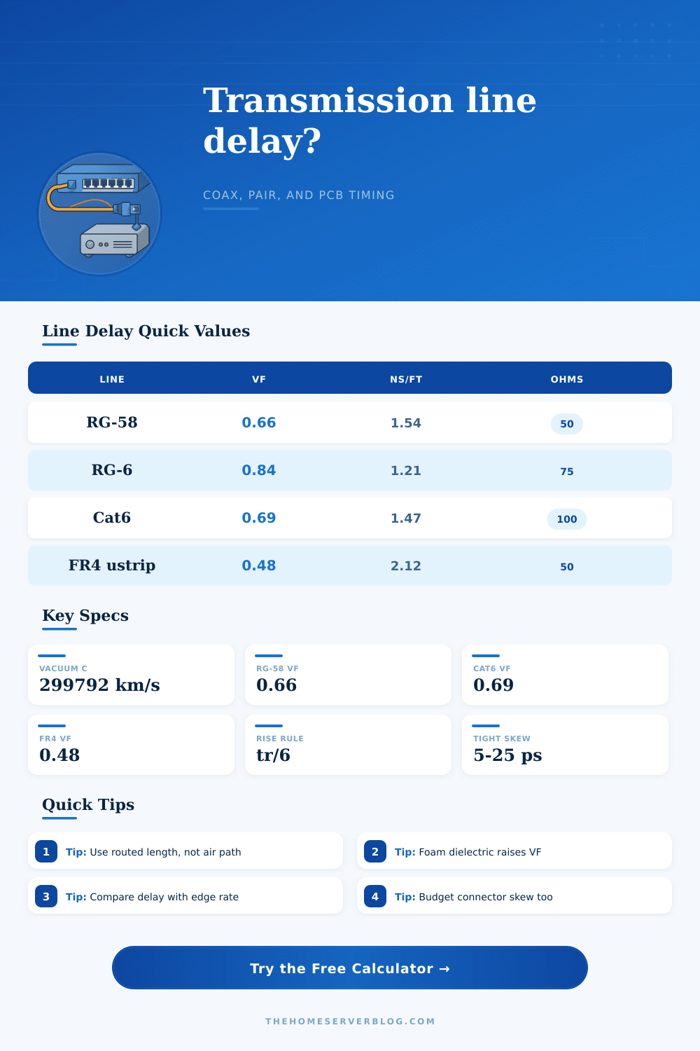
| Preset line | Typical VF | Delay per foot | Impedance | Use case |
|---|---|---|---|---|
| RG-58 solid PE coax | 0.66 | 1.54 ns/ft | 50 Ω | Bench RF, short antenna jumpers, oscilloscope leads. |
| RG-6 foam PE coax | 0.84 | 1.21 ns/ft | 75 Ω | Video, CATV, broadband, and longer low-loss runs. |
| Cat6 UTP horizontal cable | 0.69 | 1.47 ns/ft | 100 Ω | Ethernet permanent links and home-lab cabling. |
| SFP+ passive twinax DAC | 0.78 | 1.30 ns/ft | 100 Ω | Short switch, NIC, and storage interconnects. |
| FR4 outer microstrip | 0.48 | 2.12 ns/ft | 50 to 100 Ω | PCB top or bottom layer controlled-impedance traces. |
| Dielectric | Approx effective Er | Velocity factor | Delay per meter | Notes |
|---|---|---|---|---|
| Solid polyethylene coax | 2.25 to 2.30 | 0.66 | 5.05 ns/m | Classic RG-58 and many small coax families. |
| Foam polyethylene coax | 1.40 to 1.60 | 0.78 to 0.85 | 3.92 to 4.28 ns/m | Lower capacitance and faster wave speed. |
| Polyolefin twisted pair | 2.05 to 2.20 | 0.67 to 0.72 | 4.63 to 4.98 ns/m | Common for Cat5e, Cat6, and Cat6A cable. |
| FR4 microstrip | 3.2 to 3.8 effective | 0.46 to 0.56 | 5.96 to 7.25 ns/m | Outer trace fields partly travel through air. |
| FR4 stripline | 3.8 to 4.4 effective | 0.48 to 0.51 | 6.54 to 6.95 ns/m | Inner trace fields are mostly inside laminate. |
| Frequency | Quarter wave in air | VF 0.66 line | VF 0.80 line | VF 0.50 PCB |
|---|---|---|---|---|
| 10 MHz | 24.59 ft | 16.23 ft | 19.67 ft | 12.30 ft |
| 100 MHz | 2.46 ft | 19.48 in | 23.61 in | 14.76 in |
| 1 GHz | 2.95 in | 1.95 in | 2.36 in | 1.48 in |
| 10 GHz | 0.30 in | 0.19 in | 0.24 in | 0.15 in |
| Signal edge | tr/6 delay | RG-58 length | Cat6 length | FR4 length |
|---|---|---|---|---|
| 5 ns logic edge | 0.83 ns | 6.5 in | 6.8 in | 4.7 in |
| 1 ns fast edge | 0.17 ns | 1.3 in | 1.4 in | 0.9 in |
| 250 ps serial edge | 41.7 ps | 0.33 in | 0.34 in | 0.24 in |
| 50 ps very fast edge | 8.3 ps | 0.07 in | 0.07 in | 0.05 in |
Maybe you’ve wired up a circuit on a breadboard and it works, then you hook it up with a cable (or move it to a PCB) and now it doesn’t. Maybe the signal arrives late. Or it splits into echoes. Or it turns into noise. That’s annoying: on paper it seems like it should work. You checked all the voltages. You matched impedances. But what you forgot was time, Time is often the hidden issue.
It is not propagation delay. It isn’t just a number in a datasheet; it’s real-world physics. Signals actualy take time to get from one place to another. And at higher speeds they matters more than capacitance or even resistance alone.
Why Time Matters in Your Circuits
The calculator above takes care of the math for you as soon as you put in properties of your materials and the length of your cable. So you don’t need to guess how many picoseconds is hiding inside the cable. It’s a question of physics (complexly engineered). An electrical signal doesn’t move immediately. It travels as a wave guided along a conductor within an insulating material.
And how fast? All depends off what is around that copper. Light zips along at approximately 300,000 kilometers per second in vacuum. But when surrounded by solid polyethylene, it gets slowed down considerabley. When enclosed in foam insulation, it travels faster because there is plenty of air inside the insulator.
This change in speed is expressed as velocity factor. A high velocity factor indicates a quick-moving signal. A low one suggest slow going. Most designers think of it as an unchangeable constant. In truth, it vary depending on geometry and frequency. By allowing you to pick specific dielectrics such as solid PE or FR4, the tool takes into account these changes. That way, you don’t have to rely on some average number that could vary by up to ten percent. That ten percent margin of error can ruin a high-speed link.
Next think about your signal rise time. Does it take five nanoseconds for your digital edge to change? Then maybe a short cable will behave like a simple wire. With a five-nanosecond rise time, the delay isn’t even noticeable within transition window. But now shrink that rise time down to 500 picoseconds. Now each inch of trace matters. Before the signal even finishes switching, it reflect.
Here’s where electrical length diverges from physical length. You can’t eyeball a connection and know what it’ll do. You must measure it in time. That’s where the calculator comes in. It takes your physical measurements and converts them to delays. It tells you precisely how many nanoseconds or picoseconds it will take your signal to travel any distance you choose.
It also computes the quarter-wave frequency. This is the point at which your cable begins to behave more like a filter or an antenna then just a straight-through conductor.
Another issue with differential signaling is skew. Two complementary signals running down parallel traces need to reach receiver within a narrow timeframe. The larger the difference in trace length (even if caused by a different dielectric stackup), the greater the mismatch in their arrival time. At gigabit rates, a few inches of extra wire can be enough to skew data and create bit errors. By defining a maximum allowed skew budget in picoseconds, the interface will work out how much length mismatch this correspond to.
Instead of having an abstract timing requirement to worry about, you have a concrete mechanical tolerance that translates directly into the cabling or layout work you’ll do. You no longer guess whether 3 inches is too far, You know it’s over your margin.
Adding connectors introduces more delay. Whether it is a change of trace bend (pigtail), connector housings, or other specific geometries, these can changes the effective electrical length without significantly altering the physical footprint. Small differences add up fast.
Check out those reference tables comparing typical cables such as RG-58 to moddern PCB traces from the page. You’ll note that the effective dielectrics are higher for the microstrip on FR4 which makes it go much slower than foam coax. This difference dictates how you route high-speed buses versus RF feeds. High-speed bus signals. The first requires stable impedance, while the second require speed. But ultimately, it’s all about geometry in electrical clothes called timing.
Space is being shaped so that the information can come at the right time. It’s easy to overlook until the eye diagram closes or the packet loss spikes. And then you see it: Distance was never just distance. It was always delay.
Aligning the delays is what makes a prototype workable versus something that works. Because most of the trick is understanding that signal doesn’t give a damn about your schematic. All it cares about is how far it needs to walk.