Serialization Delay Calculator
Estimate packet transmit time, burst drain time, queue exit time, and effective payload throughput from frame size, link speed, L1 overhead, headers, duplex, and frame mix.
Serialization Results
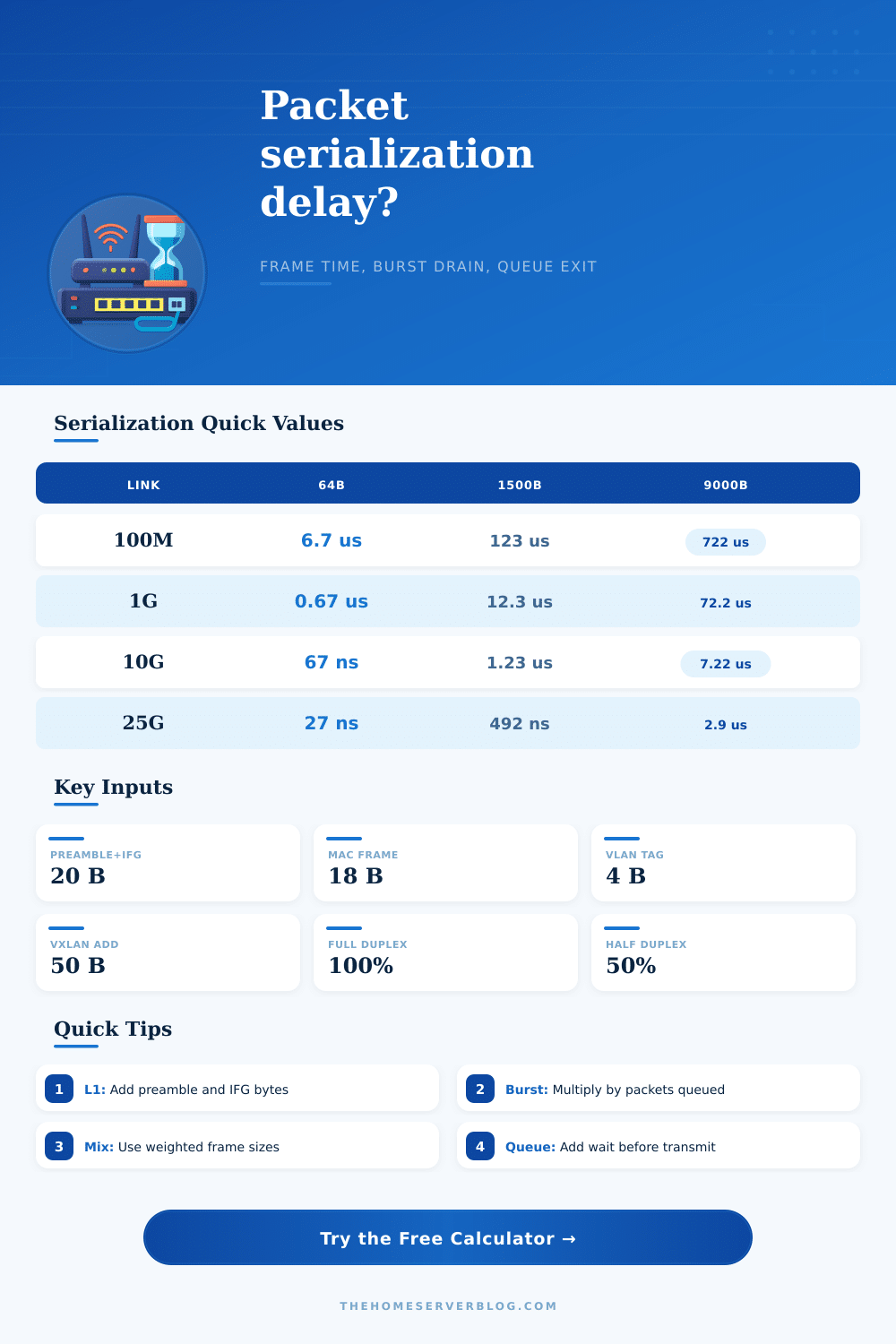
| Nominal Link | 64B Ethernet | 1500B Payload | 9000B Jumbo | 64KB Burst Frame |
|---|---|---|---|---|
| 10 Mbps Ethernet | 67.2 us | 1.23 ms | 7.22 ms | 52.5 ms |
| 100 Mbps Fast Ethernet | 6.72 us | 123 us | 722 us | 5.25 ms |
| 1 Gbps Gigabit | 672 ns | 12.3 us | 72.2 us | 525 us |
| 2.5 Gbps Multi-Gig | 269 ns | 4.92 us | 28.9 us | 210 us |
| 10 Gbps SFP+ / copper | 67 ns | 1.23 us | 7.22 us | 52.5 us |
| 25 Gbps lab spine | 27 ns | 492 ns | 2.89 us | 21.0 us |
| Component | Bytes | Usually Included In | Serialization Note |
|---|---|---|---|
| Ethernet header | 14 B | Ethernet frame | Destination, source, EtherType |
| Frame check sequence | 4 B | Ethernet frame | Transmitted after payload |
| 802.1Q VLAN tag | 4 B | Extra headers | Add once per tag |
| Preamble plus SFD | 8 B | L1 overhead | Sent before MAC frame |
| Inter-frame gap | 12 B | L1 overhead | Idle time between frames |
| Minimum Ethernet slot | 64 B | MAC frame | Pad tiny payloads to minimum |
| Traffic Pattern | Typical Size | Good Input Basis | Why It Matters |
|---|---|---|---|
| TCP ACK and control | 64 to 96 B | Ethernet frame | High packet rate, tiny serialization time |
| Standard IP data | 1500 B MTU | Payload or IP packet | Default for most home LAN tests |
| PPPoE WAN | 1492 B MTU | IP packet | Extra encapsulation lowers payload efficiency |
| VXLAN overlay | 1450 to 9000 B | Payload | Overlay bytes can push frames over MTU |
| NAS jumbo flow | 9000 B payload | Payload | Lower packet rate, longer per-frame transmit |
| Storage burst | 64 KB chunk | Bytes on wire | Useful for software queue comparisons |
| Mode | Calculator Factor | Best Use | Caution |
|---|---|---|---|
| Full-duplex dedicated | 100% | Switched Ethernet and fiber | Does not include switch fabric latency |
| Half-duplex practical | 50% | Old hubs or lab collision tests | Real collision backoff can be worse |
| Shared uplink 4:1 | 25% | Oversubscribed switch uplinks | Only an average contention model |
| Wi-Fi airtime estimate | 65% | Client airtime rough sizing | PHY rate, retries, and contention vary |
| Item | Value | Calculator Field | Home Lab Use |
|---|---|---|---|
| 1 byte | 8 bits | Frame size | All serialization math converts to bits |
| 1 Gbps bit time | 1 ns | Link speed | Fast mental estimate for gigabit LAN |
| Ethernet L1 overhead | 20 B | L1 overhead | Preamble, SFD, and inter-frame gap |
| Ethernet MAC plus FCS | 18 B | L2 header | Add when starting from payload bytes |
| Single VLAN tag | 4 B | Extra headers | Common managed switch overhead |
| VXLAN over IPv4 | 50 B | Extra headers | Overlay labs and virtual switching |
That’s where serialization delay comes in: Raw bandwidth (how fast can I send bits down a wire) is one thing; how long does it take for them to actualy get from A to B is another. On a gigabit connection, it doesn’t matter if your download speed test says 1Gig, you’ll still notice a lack of network responsiveness because serialization delay are the time it takes to physically shove bits onto a wire, not necessarily how fast they travel along it. In other words, if you’re playing an online game or making a phone call over a busy line, every single microsecond spent moving data around realy starts adding up.
But most of us begin by assuming that our network load is just the size of our application data, which we can feed into the calculator above and let it handle the math. But that presumes there’s no packaging at all, which ignores layers upon layers of stuff that gets added on top of your actual data before it even leaves the computer. There’s GRE and VXLAN tunneling protocol overhead, inter-frame gaps, frame check sequences, Ethernet headers … none of these overhead bytes contains user data, but they still consume just as much airtime as your useful packet.
Why High Speed Does Not Mean Fast Response
A seemingly harmless L1 header of 20 bytes per frame doesn’t seem like much until you’re stuffing thousands of tiny control packets down it per second. Efficiency dissapears at small frame sizes, though. What about a TCP ack that’s slightly bigger than the protocol headers around it? That one packet takes little time to serialize, but it has a horrible payload-to-wire-size ratio. You are spending almost all your link capacity moving extra data instead of real content.
This is why jumbo frames exists in storage networks; they stretch out every packet to nine thousand bytes, which spreads the cost of their overhead over more useful content. Of course, this means that each packet now take longer to send end-to-end, potentially increasing latency when the queue fills up! You can choose between lower per-packet delay or more efficient use of bandwidth, depending on your workload.
Real-world networks typically contain several types of traffic; your home network may well be running VoIP calls, IoT devices sending out heartbeats, and streaming some 4K video, all of which has varying optimal frame sizes. So the tool calculates the average serialization delay based off those weighted frame sizes to provide a more realistic picture of what’s going on instead of the theoretical best-case scenario. If you’re using half-duplex links or are operating over shared wireless channels, you can take those into account as well. Shared wireless channels causes contention and slow down the rate available for each individual stream.
When you consider what happens when 32 packets suddenly appear, they have to be sent out as a sequence, one after another, with each packet leaving the interface. Even though there might be plenty of room on the link itself, there will be a momentary increase in latency, akin to being stuck behind someone who ordered something complicated at Starbucks. (It’s not your fault you’re waiting longer, but hey, you are.) Worse, adding queued packets that arrived earlier extend this effect further. Such short-term delays is missed completely by an average-throughput measurement.
To put those delays into context: a typical fifteen-hundred-byte frame will be transmitted across a one-gigabit link in approximately twelve microseconds. On a ten-gigabit spine, that same frame is out the door in approximately 1.2 microseconds. This doesn’t seem like much when you’re transferring large amounts of data, but it’s what separates low-latency audio production from high-frequency trading.
The physics of how bits get transmitted aren’t something you can engineer around, just optimize around; match your frames to your links characteristics. It’s not about removing all delay, because you can’t, but rather anticipating where delay will occur before it affects your users. By knowing exactly how much time a packet spends on the wire, you could of avoided over provisioning hardware. You can size your buffers correctly and adjust your queue depths with precision instead of guesswork. This results in a smooth experience for latency sensitive apps.
Next time you see high bandwidth but sluggish response on your network, don’t just look at the speed test numbers; instead, check the size of the frames being transmitted. The bits might fly through quickly enough, but they could also be sitting still, waiting in line for their turn to exit. Serialization delay is hidden overhead that becomes a controllable variable once you learn about it. You then stop hunting down phantoms called ‘bandwidth’ while engineering for real-world performance.