HomeServerBlog backup operations planner
Backup Window Throughput Calculator
Estimate whether a backup job fits its maintenance window by comparing logical backup size, source read speed, target write speed, network ceiling, compression, parallel streams, dedup processing, verification pass, and operational overhead.
▣Backup window presets
⚙Window and throughput inputs
Throughput breakdown
Fit signals
📊Current backup transfer breakdown
Compressed payload sent across the selected path.
Physical bytes arriving at the repository.
Extra time from the selected verification pass.
Compressed data written before repository metadata.
🗄Backup target grid
📋Throughput and window reference tables
| Logical Size | 4 Hours | 8 Hours | 12 Hours |
|---|---|---|---|
| 1 TB | 69 MB/s | 35 MB/s | 23 MB/s |
| 4 TB | 278 MB/s | 139 MB/s | 93 MB/s |
| 10 TB | 694 MB/s | 347 MB/s | 231 MB/s |
| 20 TB | 1389 MB/s | 694 MB/s | 463 MB/s |
These rows use decimal TB and show logical data before compression, verification, or overhead.
| Path | Practical MB/s | 8-Hour Logical at 1.5x | Common Limit |
|---|---|---|---|
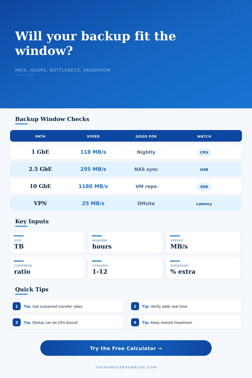
| 1 GbE | 105 to 118 | 4.5 to 5.1 TB | Link speed |
| 2.5 GbE | 250 to 295 | 10.8 to 12.7 TB | Target disk |
| 10 GbE | 900 to 1180 | 38.9 to 51.0 TB | CPU or SSD |
| VPN or WAN | 10 to 80 | 0.4 to 3.5 TB | Latency |
Compression raises logical capacity for the same wire path, but verification and retries still consume time.
| Data Type | Compression | Dedup CPU Risk | Planning Note |
|---|---|---|---|
| VM images | 1.2x to 2.0x | Medium | Changed blocks help, but active disks churn. |
| Databases | 1.1x to 1.8x | High | Dumps compress well; live images need care. |
| Photos or media | 1.0x to 1.15x | Low | Already-compressed files rarely shrink much. |
| Office files | 1.3x to 2.5x | Medium | Small files raise metadata overhead. |
Dedup processing is modeled as a logical MB/s ceiling because hashing can bottleneck before disks or links do.
| Verify Mode | Stored Bytes Read | Window Impact | Good Fit |
|---|---|---|---|
| None | 0% | Fastest | Low-risk copies |
| Metadata | 10% | Small | Nightly jobs |
| Sample | 25% | Moderate | Weekly checks |
| Full readback | 100% | Large | Cold archive |
A full readback can be correct for archives, but it may need a separate verify window.
💡Two backup window tips
It calculates duration of a backup job based off target speed and data size. That eliminates having to guess about coefficients and conversion rates.
Know your sustained throughput (the actual speed) versus theoretical link speed. In brief bursts you might get 118 MB/s through a gigabit port. However, you are not going to sustain that rate when it is hashing files, updating indexes, or verifying integrity.
How to Calculate Your Backup Time
The tool models each step of the job: reading file off the source drive, transferring over the network, writing it out to the repository, then verifying it. It models the whole job from start to finish, like a pipeline where the narrowest part of the pipe determine the overall duration.
The first bottleneck that you’ll tend to overlook is speed of your source reads. You might think “surely it’s better to have 2.5 GbE” because, well, it has a bigger number on paper, but your spinning disk array can’t necessarily feed the pipe fast enough. Even if it could, your random file access patterns will decreases the sequential throughput. If your backup set include ten thousand little documents, those disk heads will jump all around. Even at maximum pipe speed, your average speed will only be maybe forty megabytes per second.
The calculator lets you enter a realistic source speed per stream. It also considers that you may use multiple streams to help spread out the I/O load across multiple cores or physical disks. But there are diminishing returns. Ten streams doesn’t make one SATA disk go any faster. It just makes the disk work harder and run hotter.
Next you have to look at where the data’s being stored. USB external drives appear easy until cache fills up and their write speed plummets from two hundred megabytes per second down to thirty. The same goes for RAID array-based NAS storage, which slow down when computing parity.
You can see this in the chart below. It’s the typical comparison between different forms of storage. What it says is that NVMe pools aren’t typically bound by the media. They’re bound by the CPU. The CPU has to be able to feed all those flash chips fast enough while also hashing, compressing, and encrypting data. Push it too far and the CPU spikes 100 percent, the network stack starts to stutter, and boom. The job is done. And there’s the mistake folks make.
Storage isn’t just about how much. It’s about how much data can be moved over time. That saves you space, but at a cost: time. The deduplication and compression also has a limit on how much they can handle, and there is a separate field for this in the calculator. When the network fills with new data faster than your server can hash blocks, it starts backing up the queue. Even though you may have a ten-gigabit connection, maybe the CPU can only chew through two hundred megabytes per second of deduplication. That becomes your effective max. It’s a tiny factor, but one that matters if you let your job timeout just as it completes.
The moral hazard with backups is verification. Do you want to spend the time for a full readback, or do you want to cut corners and skip? The tool models both choices. A full verify pass can add hours to the job. It reads all of the bytes it wrote and verifies they matches the source. No verify means no backup. You just moved your data.
The headroom calculation will help determine whether you can afford the safety check. If estimated finish time plus verification exceeds your available window, you need either a bigger window or a faster path.
Your time is taxed by operational overhead. Catalog indexing, snapshot creation, metadata updates, retries… all of these things eat up time that isn’t reflected in the raw transfer log. Fifteen to twenty percent overhead account for that. This avoids the scenario where you plan a job which looks great on paper, but blows up in practice.
It mostly comes down to knowing what you’re measuring. Don’t just look at “bytes per second.” Look for sustained, reliable performance under load. Look in the bottleneck column when you run the numbers. That’s your answer.
Maybe you should upgrade to 2.5 GbE if that’s the network. Maybe you should add spindles or cache with SSDs if that’s the source disk. Maybe you should back off a bit on the compression level if that’s the CPU.
Remember, it’s not about running as fast as possible. It’s about completing predictably. Better to have a backup finish at 5:55 AM each night than one that finishes at 4 AM on the good nights and crashes at 8 AM on the bad ones. Make the window wide. Leave yourself headroom for the unexpected. And, oh yeah. Always check the data you thought you backed up.