HomeServerBlog optical transport planner
Dispersion Compensation Calculator
Size fixed DCM modules, estimate residual ps/nm, account for DCM insertion loss, and check whether the remaining amplifier and transceiver margins still fit a fiber span.
1Link and DCM presets
2Dispersion compensation inputs
Compensation breakdown
Planning verdict
3Live compensation cards
Raw link dispersion minus the chosen residual target.
Closest standard module count for the current span.
Compares installed compensation with the needed target cancellation.
Remaining amplifier or optical budget after module loss.
4Compensation method grid
5DCM reference tables
Common DCM module values
| Module class | Nominal compensation | Approximate SMF span | Planning note |
|---|---|---|---|
| DCM-10 | 160 to 180 ps/nm | 10 km at 1550 nm | Small correction for metro shelves, lab spools, or undercompensated routes. |
| DCM-20 | 320 to 360 ps/nm | 20 km at 1550 nm | Often fits campus extension and short metro spans with manageable loss. |
| DCM-40 | 640 to 720 ps/nm | 40 km at 1550 nm | Common fixed module size for 10G ER and DWDM metro correction. |
| DCM-80 | 1280 to 1440 ps/nm | 80 km at 1550 nm | Large correction, usually with higher insertion loss and amplifier planning. |
Fiber dispersion values by wavelength
| Fiber type | 1310 nm planning D | 1550 nm planning D | Compensation behavior |
|---|---|---|---|
| G.652 standard single-mode | 0 to 1 ps/nm-km | 16 to 18 ps/nm-km | Usually needs C-band checks beyond moderate distances. |
| G.657 bend-insensitive SMF | 0 to 1 ps/nm-km | 16 to 18 ps/nm-km | Treat like standard SMF unless the cable datasheet differs. |
| G.655 non-zero DSF | Negative to low | 3 to 6 ps/nm-km | Raw compensation need is much lower on DWDM spans. |
| DCF spool fiber | Negative | -70 to -110 ps/nm-km | Used as the compensating element, not as normal transmission fiber. |
Residual dispersion and rate sensitivity
| Rate or optic family | Typical residual concern | What to verify | Practical action |
|---|---|---|---|
| 1G and low-rate optics | Often tolerant | Vendor reach rating and power budget | Usually no fixed DCM on ordinary campus links. |
| 10G direct detect | Moderate to high | CD tolerance in ps/nm and source chirp | Use DCM near ER and ZR length classes when required. |
| 25G and 100G lanes | Higher sensitivity | Per-lane wavelength, modulation, and host FEC | Keep residual tighter and verify real module limits. |
| Coherent transport | DSP dependent | Maximum CD range, OSNR, and launch power | Often avoids fixed DCM to reduce loss and nonlinear penalties. |
DCM insertion loss and amplifier margin
| DCM plan | Typical added loss | Margin target | Operational note |
|---|---|---|---|
| Small fixed module | 2 to 4 dB | At least 3 dB spare | Good for controlled short spans if residual target is met. |
| Midspan fixed DCM | 4 to 7 dB | 4 to 6 dB spare | May need preamp or booster room depending on receiver level. |
| Stacked DCMs | 8 dB or more | Engineer per channel | Loss, nonlinear effects, and OSNR can become larger risks than CD. |
| DSP compensation | Usually no DCM loss | OSNR based | Power margin is preserved, but transponder limits still apply. |
6Field tips
One particular issue arise from chromatic dispersion in fiber optic installs. Everything looks right… The lights are on, the equipment hums along, but where’s the signal? Well, that’s the rub: There’s a signal, but it’s a garbled mess of overlaid bits the receiver can’t disentangle. Depending on its wavelength, light travel at varying speeds. A pulse of data spreads over distance. By the time it reaches far end of a given span, the bits bleed together. You can’t perceive it visually, but the error counters on your switch will let you know precisely how much that blur costs you.
To that end, I’ve created a dispersion compensation module sizing calculator (above). You plug in your desired residual target and the length of fiber to be transmitted through link. The calculator do the rest for you before you cut the cable or purchase hardware. It saves you from having to do math on conversions and coefficients yourself.
How to Fix Signal Problems in Fiber Optics
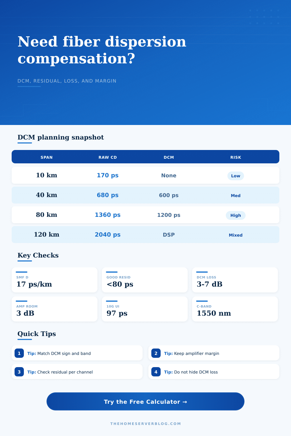
But you should of also understand what each input value mean, and how those inputs affect the outputs. Here is a quick primer: Standard single-mode fiber will gain about seventeen picoseconds of dispersion per nanometer per kilometer of transmission distance. While that may sound like a small amount, take 17 x 40 kilometers and now we’re talking about hundreds of picoseconds of accumulated delay. And if your transceiver can’t handle more than a few hundred picoseconds of delay before the eye diagram starts closing, then you have a problem. That’s the trick, knowing what it is that’s being measured.
Dispersion isn’t binary: good or bad. It’s a budget. Depending on modulation format and data rate, you have a certain amount of dispersion that you begin with. Every kilometer you push the fiber eats into that dispersion budget. Ten gigabit Ethernet is forgiving. Each bit gets a longer slice of time which can tolerates some serious dispersion. One hundred gigabit or four hundred gigabit coherent systems are far less forgiving. A smaller bit period means a smaller amount of residual dispersion can result in intersymbol interference that appears as noise to the decoder. So how much? You’ve got to know your transceiver’s tolerance before you go looking at fiber. Otherwise, you’re flying blind.
It gets complicated in other ways too with compensation. Negative dispersion compensators is known as fixed dispersion compensating modules. They are simply spools of fiber which negate the dispersion introduced by the fiber used for transmission. However, they are lossy. Adding one could increase the insertion loss on your link by four to six decibels. That’s a considerable portion of your optical power budget.
The calculator take care of that by checking the amplifier margin. In other words, it makes sure you still have enough power at end of your link after adding the compensation module. This ensures the amplifiers does not hit their noise floor or saturate. This is where folks make mistakes. They solve for dispersion, but break the power budget. You must satisfy both constraints together.
Humility about not knowing also comes into play with planning. That’s never the case that the fiber plant draw out exactly. There will be splices which introduces loss. There will be coils that extend length. And temperature will change dispersion a little bit. You can put in a percentage of uncertainty for when you plan. That isn’t pessimism, it’s engineering. A ten percent buffer is what makes up the difference between the datasheet and the digger coming back saying that the trench was realy two kilometers more than we thought from the drawing. It keeps you away from the situation where something worked well in the lab, but then fails in the field because the real world fiber length was two kilometers longer than your map implied.
Beyond fixed modules there are other options. For dynamic networks, adjustable dispersion compensating modules provides some flexibility. Coherent receivers with digital signal processing can corrects enormous amounts of dispersion without increasing physical loss. That said, there’s a limit to what DSP can do. It requires power. There is only so far it can go. Go too far, and it fails the algorithm.
On the page, you will find a list of typical module values and their matching approximations in terms of span equivalents. These can serve as a start. The objective is to reduce leftover spreading, maintaining sufficient optical margin to ensure signal remains clean. It’s a game of power vs. Timing, and when done correctly, the data flows freely. When incorrect, the deafening silence ensues.