HomeServerBlog optical transport planner
DWDM Channel Spacing Calculator
Plan dense wavelength channels from an ITU grid anchor, spacing, channel count, start offset, baud rate, rolloff, modulation, guard slots, wavelength band, and amplifier passband fit.
1DWDM presets
2Channel plan inputs
Calculation breakdown
DWDM planning verdict
3Live spacing and capacity cards
Baud rate with rolloff allowance for a single optical carrier.
Modulation estimate divided by the selected channel spacing.
First populated carrier after applying the start channel offset.
Last populated carrier at the far edge of the wavelength group.
4DWDM equipment comparison grid
5ITU grid and DWDM reference tables
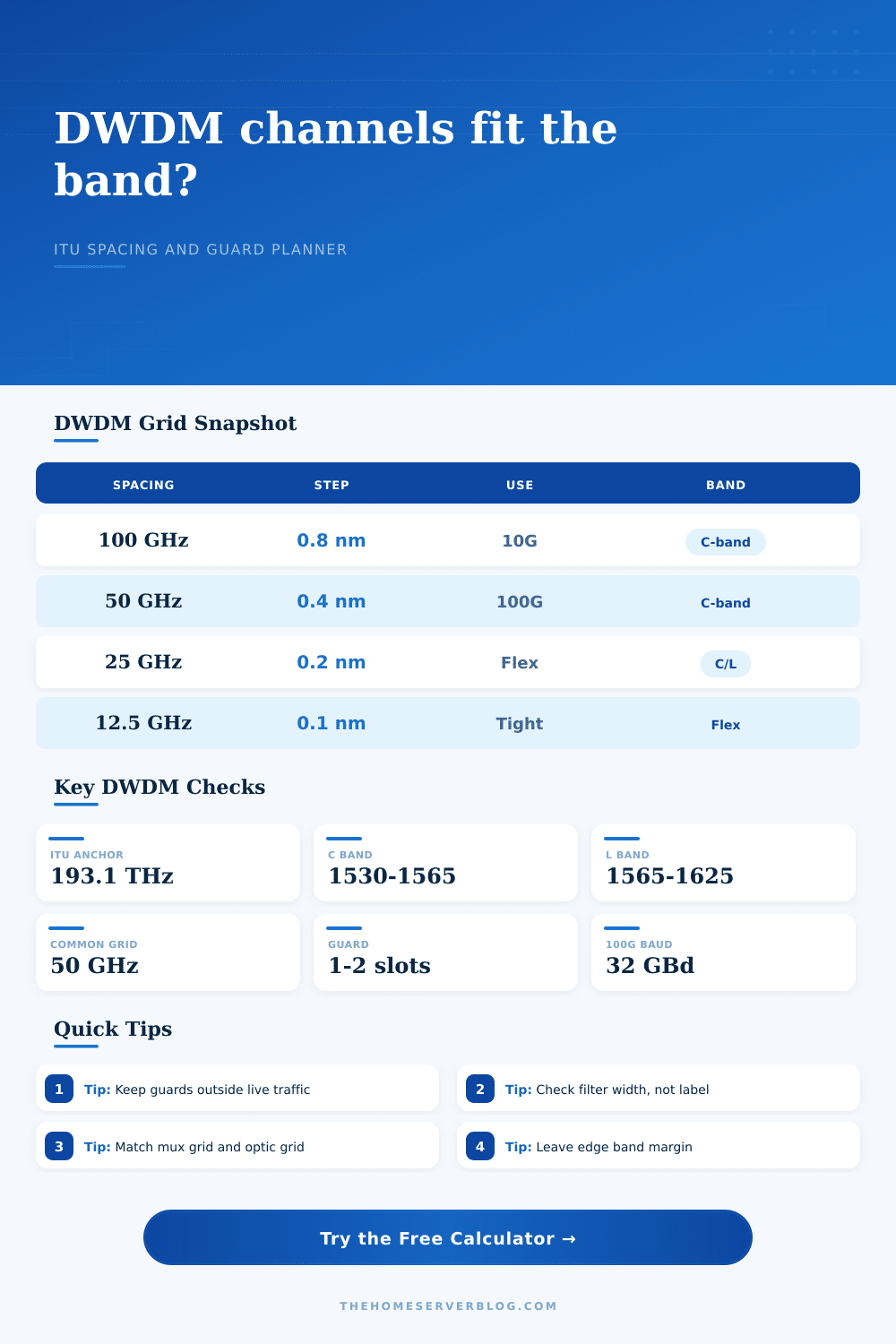
ITU-T frequency grid spacing
| Grid spacing | Frequency step | Approx nm near 1550 | Typical planning use |
|---|---|---|---|
| 100 GHz | 0.100 THz | About 0.80 nm | Classic fixed-grid 10G, 40G, simple mux shelves. |
| 50 GHz | 0.050 THz | About 0.40 nm | Common 80-channel C-band plans and coherent 100G. |
| 25 GHz | 0.025 THz | About 0.20 nm | Narrow fixed grid or flex-grid building block. |
| 12.5 GHz | 0.0125 THz | About 0.10 nm | Flex-grid slot granularity, not always a standalone mux pitch. |
ITU anchor examples around 193.1 THz
| Offset n | Frequency | Wavelength | 50 GHz channel note |
|---|---|---|---|
| -4 | 192.900 THz | 1554.94 nm | Longer wavelength side of anchor. |
| -2 | 193.000 THz | 1554.13 nm | Near center C-band reference. |
| 0 | 193.100 THz | 1553.33 nm | Classic ITU reference frequency. |
| +2 | 193.200 THz | 1552.52 nm | Shorter wavelength side of anchor. |
| +4 | 193.300 THz | 1551.72 nm | Still inside the usual C-band window. |
Wavelength and amplifier bands
| Band | Approx wavelength | Approx frequency | Planning note |
|---|---|---|---|
| C-band | 1530 to 1565 nm | 195.9 to 191.6 THz | Most common EDFA-backed DWDM operating window. |
| Extended C | 1528 to 1568 nm | 196.2 to 191.2 THz | Needs compatible mux, WSS, and amplifier gain flattening. |
| L-band | 1565 to 1625 nm | 191.6 to 184.5 THz | Used when capacity expands beyond C-band shelves. |
| C plus L | 1530 to 1625 nm | 195.9 to 184.5 THz | Usually separate C and L amplifier chains or open line gear. |
Baud rate fit by spacing
| Spacing | Comfortable width | Borderline width | Typical signal example |
|---|---|---|---|
| 100 GHz | Under 75 GHz | 75 to 90 GHz | High-baud 400G, legacy 10G with wide filters. |
| 75 GHz | Under 56 GHz | 56 to 67 GHz | Coherent 400G with moderate rolloff. |
| 50 GHz | Under 38 GHz | 38 to 45 GHz | 32 GBd coherent or tuned 100G waves. |
| 25 GHz | Under 19 GHz | 19 to 22 GHz | Narrow-band low-baud transport channels. |
6Planning tips
Fiber optics often feels like magic until you try to pack more data onto a single strand then it seems capable of holding. Typically, you’ve got some plan in mind, double your capacity on that transport without digging up the street and laying new cable, for instance. The answer is typically “add more wavelengths”, which mean you need to make room in the glass. But that brings a messy problem of spectral real estate. Light doesn’t care what your target bandwidths are; it’s governed by physics. Physics require strict spacing to prevent channels from bleeding into each other, so you had better have a good idea of how much space every signal occupy.
That’s where the calculator comes in. The one up top do the math for you, converting those basic ITU grid numbers into a real map of your optical link. You can see if your planned channels fall within useful range of your amplifier, or if your chosen modulation scheme leaves sufficient safety margins.
How to Plan Your Optical Network
We all know the anchor frequency for the C-band is 193.1 THz, but who remembers that’s merely a reference point within a large sea of frequencies? All that really matter are the channels you arrange themselves around it. The initial decision that actualy matters is determining the right channel spacing. The default grids is 100 GHz, 50 GHz and in some cases 25 GHz. The wider-spacing make things simple for amplifiers and filters, lots of clear spectrum between each signal. The narrower-spacing stuffs more channels onto a single fiber. So if all else is equal, it dramatically increases overall capacity. That’s the whole of the game: Tighten up the grid to get more bandwidth but lose flexibility.
If the occupied width of your signal is greater then or equal to the grid spacing, then your signals starts interfering with the adjacent ones. This increase errors and kills your data. Don’t forget to consider the filter rolloff and baud rate. Just because the data rate is 32 GBd doesn’t mean that the signal occupy a full 32 GHz of bandwidth. The rolloff factor adds extra width to include the signals side lobes. The shape of the signal also matter. Failing to take this additional width into consideration is a frequent error resulting in crosstalk. This occupied width is calculated by tool for you and compared with your selected spacing, indicating whether or not you’re cutting it too close. When the occupancy reaches 90 percent of the slot, you’re pushing your luck.
The other non-negotiable item in a good plan is use of guard channels. Guard channels are empty slots reserved at the edges of your channel group to protect against amplifier tilt, blocker filter rolloff, and future expansion. Not leaving any guards will get you maybe a couple gigahertz more right now, but it will leave you nowhere to grow and adjust your power levels and add additional waves. Waste a channel now; you should of rethink the entire link next year.
One thing that’s easy to forget until the light is red is amplifier compatibility. Most amplifiers operate in a particular passband, typically within the C-band (i.e., wavelengths between 1530-1565 nm). Any channels that is off this window won’t be boosted as well by the amplifier, causing signal power loss toward the ends of your channel plan. The chosen amplifier band is compared against your wavelength range; any channels not within the usable part of the gain region gets flagged. Don’t embarrass yourself by provisioning channels that won’t reach other end.
Last, keep in mind that the king is spectral efficiency. Using higher-order modulation such as DP-16QAM (or even DP-64QAM) means packing more bits into each symbol, which enables you to fit more within a narrow slot while maintaining the same data rate. These formats are also more susceptible to crosstalk and noise. You need excellent dispersion management and clean fiber conditions to pull it off with tight spacing. It works, but it require precision.
The number of wavelengths isn’t the only consideration in planning out a DWDM network. There’s the stuff that goes on between them too; how close they can be before their signals gets garbled. You’re trading off operational stability against raw capacity. How much breathing space does each of these signals need? If you don’t have this right, you’ll end up with a dark fiber link that’s intermittently error-prone, or one that just works fine year after year. Respect the guards, start with the grid and always double-check the edges. It is simple math, but there are expensive consequences if you get it wrong.