DynamoDB Read Capacity Calculator
Estimate DynamoDB read capacity units from item size, eventual and strong consistency, transactional reads, read rate, burst headroom, GSI fanout, DAX or cache hit rate, and table mode.
Capacity Breakdown
| Item Size | 4 KB Units | Eventual Read | Strong Read | Transactional Read |
|---|---|---|---|---|
| 1 KB to 4 KB | 1 | 0.5 RCU | 1 RCU | 2 RCUs |
| 4.1 KB to 8 KB | 2 | 1 RCU | 2 RCUs | 4 RCUs |
| 8.1 KB to 12 KB | 3 | 1.5 RCUs | 3 RCUs | 6 RCUs |
| 12.1 KB to 16 KB | 4 | 2 RCUs | 4 RCUs | 8 RCUs |
| 16.1 KB to 32 KB | 5 to 8 | 2.5 to 4 | 5 to 8 | 10 to 16 |
| 32.1 KB to 64 KB | 9 to 16 | 4.5 to 8 | 9 to 16 | 18 to 32 |
| Consistency Mode | Multiplier | Freshness | Allowed Target | Capacity Note |
|---|---|---|---|---|
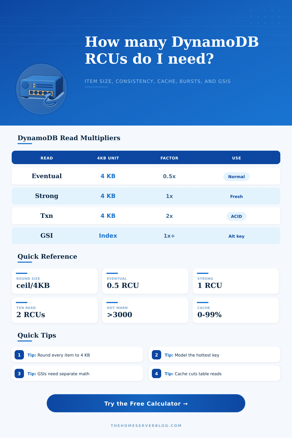
| Eventually consistent | 0.5x | May lag briefly | Table and GSI reads | Lowest RCU load for normal read paths |
| Strongly consistent | 1x | Latest committed data | Table and LSI reads | Not available on global secondary indexes |
| Transactional read | 2x | ACID transaction view | Transaction APIs | Use for workflows that need transaction semantics |
| DAX or app cache hit | 0x table | Depends on cache policy | Cacheable items | Reduces reads that reach DynamoDB |
| Read Pattern | Best Consistency | Use When | Watch Metric | Optimization |
|---|---|---|---|---|
| Profile or catalog lookup | Eventual | Small freshness lag is acceptable | Cache hit rate | Add DAX or local cache |
| Post-write confirmation | Strong | User must see latest write | RCU spike after writes | Use strong reads only on confirm path |
| Financial workflow | Transactional | Multiple items must be read consistently | Txn read volume | Keep transaction item count small |
| Leaderboard by score | Eventual on GSI | Alternate key access is needed | GSI consumed capacity | Project only fields needed by read |
| Admin audit viewer | Strong or eventual | Freshness depends on operator need | Scans and page size | Prefer key queries over scans |
| Planning Area | Good Signal | Warning Signal | Practical Response |
|---|---|---|---|
| Provisioned mode | Target utilization below 70% | Consumed RCUs near provisioned limit | Raise RCUs or tune auto scaling target |
| On-demand mode | Traffic ramps gradually | Sudden large read surge | Warm up traffic and fix hot keys |
| GSI reads | Projected item is small | Index item is larger than table item | Use narrower projections for read-heavy GSIs |
| DAX or cache | High hit rate on repeat reads | Low hit rate with high churn | Review TTL, key design, and invalidation |
| Hot partition | Hottest key below partition budget | One key group carries peak traffic | Shard key, bucket time, or spread reads |
DynamoDB tables can choke under their own success. It isn’t necessarily due to a sudden spike in traffic; it can be caused by things like consistency settings or hot partitions. Naturaly it isn’t because you’ve suddenly gotten more requests; it’s usually because your consistency setting are wrong. Your average load might work fine with one table, while peaking loads causes that same table to crash when every page view demand strong consistency. Read capacity is paid for by cost of accurate data, milliseconds for money.
Engineers generaly view Read Capacity Units as a straight traffic multiplier and ignore that their pricing depend on their consistency model. Eventually consistent reads can be low-cost because they permit some delay; strongly consistent ones needs to check multiple replica, thus doubling the cost per item. Transactional reads cost 4x the price of eventual reads due to atomic guarantees. Break your read traffic into those three categories and then look at actual cost: you’ll discover not all reads costs alike.
How to Save Money on DynamoDB Reads
Another hidden cost is the size of items, since DynamoDB bills for data in four-kilobyte blocks. So if your item is slightly bigger than 4KB, say 4.5 KB. It will be treated as two unit of capacity, regardless of how much data you’re actualy getting back. The result is that smaller items increases the efficiency of reads (as well as storage), since they consume fewer blocks per request. When dealing with millions of requests, optimizing item size can matter, because although you may believe you’re reading tiny pieces of data, the billing engine think you’re doing some heavy lifting.
But then there’s caching, which changes everything by avoiding most reads to DynamoDB. By storing common answers in memory (e.g., via DAX or a local app cache), you can enter the hit percentage into calculator. If 35% of your traffic is cached, then only 65% will be using Read Capacity Units. Because you forget about caching, you tend to over-provision, paying for resources that are unused if they’re already sitting on your server. By the way, this also helps make the DynamoDB pricing more predictable: it help you match capacity to reality so you don’t pay for idle resources during lulls.
Reads get much more complex with Global Secondary Indexes, which will use capacity of both base table as well as the index. An index that projects more fields than it need will increase the RCU cost and also cause your items to be larger. Because a GSI read may be costly due to inclusion of large attributes, you need to model that separately. Check reference table on the page to see how each consistency mode maps to its multiplier. This would of help you see why some reads cost more then you might expect.
Partition hot spots are still very important: The size of your total furnitures is irrelevant if all the traffic hits a single partition key. Because DynamoDB distributes data across multiple partitions, a skewed pattern of access will cause a single shard to handle all the traffic; with other shards idle. There’s no way to fix that with additional Read Capacity Units; instead you need to address it in design by sharding keys or distributing writes over time. The calculator has a check for this risk and flags you when a single key accounts for too large portion of the traffic.
If your traffic is unpredictable, go with on-demand mode. You pay more per unit of usage, but you don’t get throttled. Otherwise, choose provisioned capacity and tune your auto-scaling policy so you has enough capacity in steady state. The tool will also let you label your mode, which changes the recommendation logic. Based off that option, it will change the advice provided. For hobby projects with sporadic traffic, go with on-demand. For high-throughput catalogs, go with provisioned capacity but carefully limit your scaling to save money.
Now, don’t try to shoehorn Read Capacity Units down as low as possible; we’re simply aiming to match capacity to the real world here. Begin with an estimate of peak load and use a usage target on top of that. Typically, 70% is a good compromise, it lets you have some “headroom” for unexpected spikes, but doesn’t waste money when things are quiet. The key with DynamoDB is that you has to think about design in terms of access patterns (not just where it’s stored), and each read decision is a tradeoff among latency/cost/consistency. Once you get your head around that tradeoff, then the numbers makes sense and you don’t guess at performance anymore. For example, that earlier session data didn’t require strong consistency. It just had to look like it was fresh. In some cases, good enough is actualy good enough.