EIGRP Bandwidth Delay Metric Calculator
Calculate classic EIGRP composite metrics from minimum bandwidth, cumulative delay, K-values, load, reliability, MTU, offset lists, and variance-ready path comparisons.
| Path model | Bandwidth | Delay | Metric | Result |
|---|---|---|---|---|
| Current input | 1544 Kbps | 20000 us | 2172416 | Successor candidate |
Common interface bandwidth and delay defaults
| Interface or link | Bandwidth used | Typical delay | Default metric with K1/K3 |
|---|---|---|---|
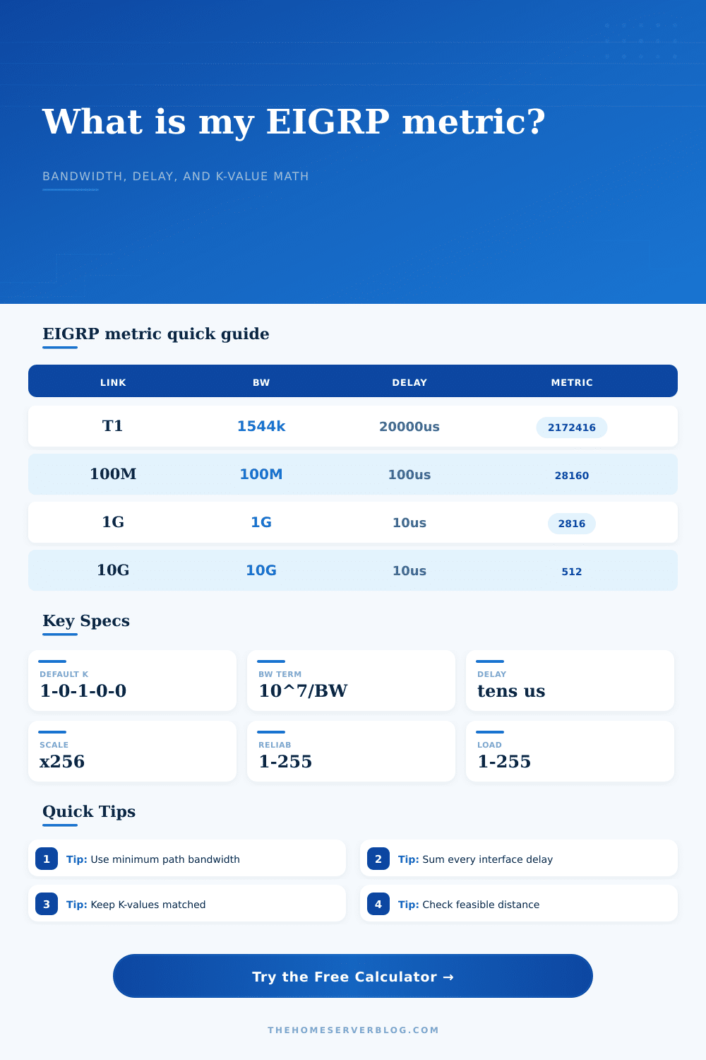
| Serial T1 | 1544 Kbps | 20000 microseconds | About 2,172,416 |
| Ethernet 10M | 10000 Kbps | 1000 microseconds | About 281,600 |
| FastEthernet 100M | 100000 Kbps | 100 microseconds | About 28,160 |
| GigabitEthernet | 1000000 Kbps | 10 microseconds | About 2,816 |
| 10 GigabitEthernet | 10000000 Kbps | 10 microseconds | About 512 |
EIGRP metric and K-value comparison grid
| Profile | K-values | Formula emphasis | Operational note |
|---|---|---|---|
| Cisco default | K1=1 K2=0 K3=1 K4=0 K5=0 | Bandwidth plus delay | Most common and easiest to reason about |
| Delay-only lab | K1=0 K2=0 K3=1 K4=0 K5=0 | Cumulative delay only | Useful for demonstrations but rare in production |
| Load-aware | K1=1 K2=1 K3=1 K4=0 K5=0 | Bandwidth, load, delay | Can cause route movement as interface load changes |
| Reliability-aware | K1=1 K2=0 K3=1 K4=0 K5=1 | Reliability multiplier | Needs careful neighbor-wide agreement |
| Wide metric mode | Named EIGRP families | Larger metric scale | Better precision on high-speed links |
Bandwidth term sensitivity
| Minimum bandwidth | Bandwidth term | Delay example | Metric effect |
|---|---|---|---|
| 1544 Kbps | 6476.68 | 20000 microseconds gives 2000 | Slow WAN bandwidth dominates |
| 10000 Kbps | 1000.00 | 1000 microseconds gives 100 | Older Ethernet still noticeable |
| 100000 Kbps | 100.00 | 100 microseconds gives 10 | Metric falls sharply at FastEthernet |
| 1000000 Kbps | 10.00 | 10 microseconds gives 1 | Delay begins to matter more |
| 10000000 Kbps | 1.00 | 10 microseconds gives 1 | Classic metric has coarse precision |
Common home lab and branch scenarios
| Scenario | Minimum bandwidth | Cumulative delay | Routing lesson |
|---|---|---|---|
| Proxmox lab core | 1 Gbps | 20 microseconds | Both paths may look nearly equal |
| Firewall to ISP CPE | 100 Mbps | 1000 microseconds | Bandwidth and delay both influence path |
| DMVPN branch tunnel | 20 Mbps | 30000 microseconds | Delay tuning can prevent poor hub choices |
| LTE backup route | 10 Mbps | 80000 microseconds | High delay should keep it as backup |
| Metro-E ring | 1 Gbps | 200 microseconds | Small delay differences can rank paths |
The single biggest mistake people make with routers is looking at link speed, thinking their router automatically figures out what to do with it. While EIGRP can be smart, it’s also rigid. It doesn’t care about theoretical maximums or marketing specs; it cares about total lag of every interface along the path plus speed of slowest hop. That’s what you have to think about when you’re trying to determine what a router pick as its best route… think like the algorithm, not the network diagram.
Once you understand your real-world constraints, enter them into the calculator above and let it handle the math for you… including saving you from guessing how all those coefficients work together behind-the-scenes.
How EIGRP Chooses the Best Route
The classic metric is also deceptively simple, it combines bandwidth and delay. And here’s the problem, the bandwidth part of that formula follows bottleneck principle. If your LAN connection is a gigabit and your WAN connection is a twenty-megabit, then the route will be treated as if it’s a twenty-megabit route. High speed internal routes don’t cover up slow external ones. EIGRP identifies weakest link in the chain and treats entire route based off that link. The result is that the routing protocol honors the real capability of the exit link, and doesn’t flood it with traffic because core is fast.
The second part is other side of that coin: Delay. Unlike Bandwidth, where the lowest number wins, Delay is cumulative. Each link the packet traverses add its own delay, and typically engineers forget about it since moddern interfaces are super fast. But in a multi-hop scenario, these little bits get cumulative, and a couple hundreds micros here and there can tip the metric just enough to cause a route switch. The calculator will show you that accumulation, and you can also change the delay values to vary your path length to see what happens to the metric at the end. It’s why sometimes a longer physical path may win out due to lower configured delays on the intermediate links.
The other thing to know about K-values is that they determines what’s important. By default, K1 is set to bandwidth and K3 is set to delay; the rest are 0. So, without changing those, only bandwidth and delay matter. Why? Because you also don’t have K-values set for load and reliability. But changing the K-values can be tricky. Everyone within your autonomous system has to agree on K-values. If one router determine that load is an important factor but another doesn’t, they won’t form a stable adjacency. The neighbor relationship falls apart and you lose the route. That’s why the calculator takes K-values into account. You can play around with various sets of them without actualy modifying your production gear. You’ll get to see how turning on K2 or K5 changes path selection without affecting network stability.
The rule that makes it possible for routes to be loop free is called feasible distance. To check whether a route is a valid backup, you have to compare it to your own feasible distance of that route; in other words, the reported distance back from your neighbor has to be less than yours. That’s what keeps routing loops out, your neighbor isn’t getting its traffic back via you to get to where they came from. If there’s a possibility of an alternate route that does that, the tool lets you know and won’t let you use it. That’s key when trying to make sure something else can come online as soon as something else fails. You don’t want a backup route that creates blackholes.
Tuning delay is clean. It doesn’t mess with your monitoring tools or QoS policies because it’s simply modifying the routing metric. A little goes a long way… If you’re trying to favor one path over another, then you modify the delay on that interface. The calculator tells you precisely what needs to be changed in order to flip the preference. It takes the guesswork out of determining which path to pick.
Another tool is offset lists which adds a penalty to the metric after it’s calculated. Use this to fine tune routing without having to change interface parameters, for example, if a given route would be fast but cross through a busy area. You could penalize that path. You enter offsets into the calculator and see what effect the penalty have on the final metric. This allows you to plan complex policy decisions ahead of time.
Theory assumes that links remain stable and synchronized perfectly. Reality is that interfaces flap and congestion varies in real networks. EIGRP tries to account for this in the way it calculates metrics, and it attempts to balance latency and speed while favoring stability. While the math may seem complex, having an understanding of it will allow you to predict behavior and work WITH the protocol rather than against it.
The calculator allows you to play in a sandbox and test those concepts. It also lets you convert those abstract concepts into concrete numbers. It lets you see the effects of your design decisions and prove your assumptions. That kind of knowledge is priceless. It differentiates the engineers who design networks from the technicians who simply configure routers. You don’t want just connectivity, you want traffic to flow efficiently and predictably. When you know how the metric was constructed, you have the ability to affect that traffic flow and understand what controls the cost. THAT is why we should of done the exercise.