HomeServerBlog distributed storage planner
Erasure Coding Overhead Calculator
Estimate usable capacity, parity overhead, safe fill, logical capacity after compression, fault tolerance, rebuild read load, and rebuild time for k+m erasure coded home lab storage pools.
▦Erasure coding presets
⚙Erasure coding inputs
Capacity breakdown
Health and rebuild reading
▣Calculated capacity markers
Total participating drive capacity before parity or reserves.
Complete groups times k data shards times per-drive capacity.
Complete groups times m parity shards times per-drive capacity.
Drives outside complete k+m groups unless your platform spans groups differently.
⚒Equipment and media comparison grid
NAS HDD 5400/5900
95 MB/sQuiet capacity drives with lower rebuild speed. Useful for media pools and small always-on storage.
NAS HDD 7200
145 MB/sBalanced home lab choice. Higher sequential rebuild rate but more heat and vibration than slower disks.
Enterprise HDD
185 MB/sBetter sustained rebuild behavior and workload rating. Watch idle watts in a small rack.
SMR Archive HDD
45 MB/sCapacity-focused media can rebuild slowly during random rewrites, compaction, or backfill.
SATA SSD
420 MB/sPredictable small-block recovery with SATA bus limits. Endurance reserve matters for write-heavy pools.
NVMe SSD
1200 MB/sFast rebuild math, often limited by network, CPU coding work, or PCIe topology.
USB Backup HDD
75 MB/sGood for portable vaults, less ideal for always-on degraded recovery due to bus and enclosure limits.
Mixed Used Drives
65 MB/sModel using the smallest and slowest member when old disks share one stripe group.
ℹReference tables
Capacity by k+m layout
| Layout | Raw efficiency | Parity overhead | Best use |
|---|---|---|---|
| 3+2 | 60.0% | 66.7% over data | Small clusters, high protection per node. |
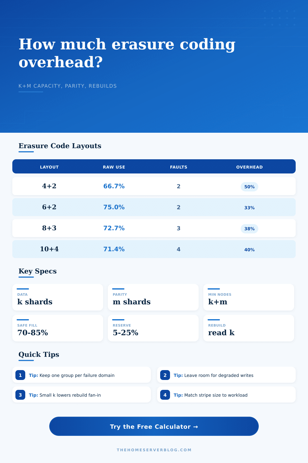
| 4+2 | 66.7% | 50.0% over data | Common six-drive or six-node home lab groups. |
| 6+2 | 75.0% | 33.3% over data | Good balance for eight-drive NAS shelves. |
| 8+2 | 80.0% | 25.0% over data | Capacity-heavy media with reliable hardware. |
| 8+3 | 72.7% | 37.5% over data | Large disks where rebuild exposure matters. |
| 10+4 | 71.4% | 40.0% over data | Wide archive groups with four-shard tolerance. |
Drive capacity conversions
| Drive label | Approx TiB | 4+2 usable | 6+2 usable |
|---|---|---|---|
| 4 TB | 3.64 TiB | 16 TB / 14.6 TiB | 24 TB / 21.8 TiB |
| 8 TB | 7.28 TiB | 32 TB / 29.1 TiB | 48 TB / 43.7 TiB |
| 12 TB | 10.91 TiB | 48 TB / 43.7 TiB | 72 TB / 65.5 TiB |
| 18 TB | 16.37 TiB | 72 TB / 65.5 TiB | 108 TB / 98.2 TiB |
| 22 TB | 20.01 TiB | 88 TB / 80.0 TiB | 132 TB / 120 TiB |
| 30 TB | 27.28 TiB | 120 TB / 109 TiB | 180 TB / 164 TiB |
Rebuild and backfill planning
| Media profile | Model rate | Efficiency | Planning note |
|---|---|---|---|
| NAS HDD 5400/5900 | 95 MB/s | 70% | Quiet pools need longer degraded windows. |
| NAS HDD 7200 | 145 MB/s | 75% | Balance rate against heat and vibration. |
| Enterprise HDD | 185 MB/s | 80% | Better for heavy scrub and recovery cycles. |
| SMR Archive HDD | 45 MB/s | 55% | Avoid heavy degraded random write workloads. |
| SATA SSD | 420 MB/s | 82% | Often limited by controller or network path. |
| NVMe SSD | 1200 MB/s | 75% | CPU coding or network fan-in can dominate. |
Common project sizes
| Project | Layout | Raw pool | Safe result |
|---|---|---|---|
| Six-bay mini cluster | 4+2 | 48 TB | About 21 to 24 TB logical. |
| Eight-bay home NAS | 6+2 | 96 TB | About 48 to 56 TB logical. |
| Ten-disk media shelf | 8+2 | 180 TB | About 105 to 120 TB logical. |
| Triple-parity photo lab | 8+3 | 220 TB | About 115 to 130 TB logical. |
| Dual archive groups | 10+4 | 504 TB | About 260 to 300 TB logical. |
| Small edge nodes | 3+2 | 20 TB | About 8 to 10 TB logical. |
⚡Home lab planning tips
This calculator models erasure coding at the planning layer. Real platforms may reserve additional space for placement groups, object size rounding, journals, snapshots, compression dictionaries, checksums, or minimum allocation units.
After you’ve got a bunch of disks stuffed inside a server chassis, how many are left over? And what’s the server holding back as part of the file system protection?
If you use erasure coding, it’ll break up your data into shards that get spreaded out onto different disks. So if some goes missing, you won’t lose your files. But there’s no free lunch here. Rebuilding from scratch takes time, and there’s an overhead cost in terms of matching. Raw disk capacity comes with a price tag, too.
How to Use the Erasure Coding Calculator
Plug in your number of drives and type of coding on top and the calculator will work the numbers out for you… No need to guess at what conversion factor or coefficient applies.
K plus m is the core idea here. K equals the data shards containing your real data. M equals the parity shards needed for rebuilding when a drive go down. A typical home lab deployment will use four drives for data and two for parity. That’s sixty-six percent efficiency, i.e., two-thirds of available disk space. But amount of parity data used to protect information is 50% larger.
By moving to a six plus two layout, you achieve seventy-five percent efficiency. You get more bang for your buck on parity. But more expense during rebuild: Each time a drive die in a six plus two stripe set, the system needs to draw from five surviving data drives to rebuild. It is efficient at rest but expensive in motion.
But also take into account what kind of media it’s going to be. A fast seven-thousand-two-hundred RPM enterprise disk will rebuild far faster than a slower five-thousand four-hundred RPM NAS drive. These throughput numbers can vary widely. According to the table on the page, a mechanical drive could rebuild as slow as ninety-five megabytes per second, while an NVMe SSD can reach one thousand two hundred.
Why does this matter? Because the longer your rebuild takes, the higher your chance of having another drive fail before the initial one has been fixed. If you have a big parity group rebuilding over a long time and two drives goes down in the process, you’re out of luck. This is why calculator asks for both a degraded rebuild reserve and target maximum fill percentage.
I’m not being conservative when I leave my pool 80% full. This leaves room for storage engine to breathe. To do garbage collection of SSDs. It handles metadata updates. It also performs backfill operations where data are moved around in distributed systems. If you pack every terabyte without leaving any space, the system slows down as it looks for empty slots where it can write its new parity information.
Another strong way is adding a compression ratio. If you’re storing un-compressed video, databases or text logs, then you may get a ten percent gain. But if you are already compressing media files or want to encrypt backups, the ratio doesn’t change. It stays one to one, which means capacity is actualy what the math says.
What about layout? You will want different layouts depending on the type of failure you expect in your fault domain. If you’re storing a media archive and don’t change much, you can get four-shard tolerance and huge capacity by going 10 plus four. It takes ten drives, but they all function as a single unit.
If space isn’t an issue, then go with safety: 3 plus 2 protects against two drives in a very small subset failing at once. If you have a busy home server that does lots of writes, go with a lower k, it’ll keep the write penalty down. If you’re doing more long-haul stuff, go with a higher m and rest easy knowing that you’ve got some peace of mind.
The tool also figures out how long it would of take to rebuild one shard, so you can kind of visualize how long that’s taking. That makes a difference when planning your maintenance windows, too. It could be a six-hour rebuild instead of a 12-hour rebuild.
In conclusion, erasure coding means sacrificing some space to make it safer. Storage is not free. You can’t get maximum speed + maximum safety + maximum density, you’ve got to choose two. Play with the presets; they’ll show you what impact various profiles have on the numbers. Try a deep archive vault versus a mini Ceph cluster, and look at how the usable capacity scales when the parity changes in size.
The point here is to configure a pool that withstands expected hardware failure while not forcing you to buy more disk space than you wanted. Begin with real-world hardware inputs, tweak the fill levels based off comfort, and then let the numbers inform your buying decisions. Your data will appreciate the foresight.