EtherChannel Bandwidth Calculator
Estimate raw bundle bandwidth, hash-adjusted usable capacity, failover impact, and single-flow limits for LACP, PAgP, and static link aggregation groups.
Calculated LAG capacity
These values update after each calculation and are meant for quick comparison while you change port counts, speeds, and failure assumptions.
Small smart switch
Often supports static LAG and basic LACP with limited hash choices. Best for NAS and AP pairs where the traffic pattern is predictable.
Cisco Catalyst style
Commonly supports LACP, PAgP, source/destination IP, and Layer 4 port hashing. Strong choice for mixed clients and server VLANs.
Aruba / ProCurve style
LACP is typical, with trunk groups and configurable load distribution. Good fit for home lab cores and access switch uplinks.
MikroTik / RouterOS style
Bonding modes vary by hardware offload support. Check bridge offload before assuming line-rate routing or switching through the bundle.
| Mode | Negotiation | Good use | Calculation note |
|---|---|---|---|
| LACP active/passive | IEEE 802.3ad / 802.1AX negotiation | Most NAS, server, and switch uplinks | Fast failure detection; calculate active links minus failed links. |
| PAgP desirable/auto | Cisco proprietary negotiation | Older Cisco-only environments | Similar bandwidth math, but both ends must support PAgP. |
| Static on/on | No negotiation | Simple lab links when both sides are fixed | Can blackhole traffic if one side is miswired or mismatched. |
| Manual balance | Platform-specific bonding | Router or Linux bonding tests | Verify hardware offload and switch compatibility before trusting totals. |
| Hash mode | Fields used | Best traffic pattern | Risk to watch |
|---|---|---|---|
| Layer 2 MAC | Source and destination MAC | Many local clients crossing one access switch | Router-on-a-stick traffic can collapse onto fewer members. |
| Layer 3 IP | Source and destination IP | Many VLANs, many clients, routed storage networks | One big host-to-host transfer still uses one member. |
| Layer 4 ports | IP addresses plus TCP/UDP ports | SMB multichannel, web, backup, and VM traffic | Encrypted tunnels may hide individual flows from the switch. |
| Adaptive / flowlet | Vendor load signal or flowlet timing | Modern data center or high-end switch fabrics | Not available on many home lab switches. |
| Bundle example | Raw aggregate | One-flow ceiling | Common use |
|---|---|---|---|
| 2 x 1G | 2 Gbps | About 1 Gbps | Small NAS or firewall pair |
| 4 x 2.5G | 10 Gbps | About 2.5 Gbps | Wi-Fi 6 AP aggregation or desktop edge |
| 4 x 10G | 40 Gbps | About 10 Gbps | Proxmox storage, NAS, lab core |
| 8 x 25G | 200 Gbps | About 25 Gbps | Switch stack, high-density host uplink |
| Scenario | Flow count clue | Target utilization | Practical sizing note |
|---|---|---|---|
| NAS file serving | Clients plus SMB channels | 70% to 80% | Enable SMB multichannel when both client and NAS support it. |
| Proxmox cluster | VMs, replication, storage sessions | 60% to 75% | Separate corosync from heavy storage where possible. |
| AP aggregation | Client sessions per AP | 75% to 85% | Wireless airtime is usually the limit before uplink bandwidth. |
| Core uplink | Many VLAN conversations | 65% to 80% | Use IP plus port hashing if most traffic crosses routed boundaries. |
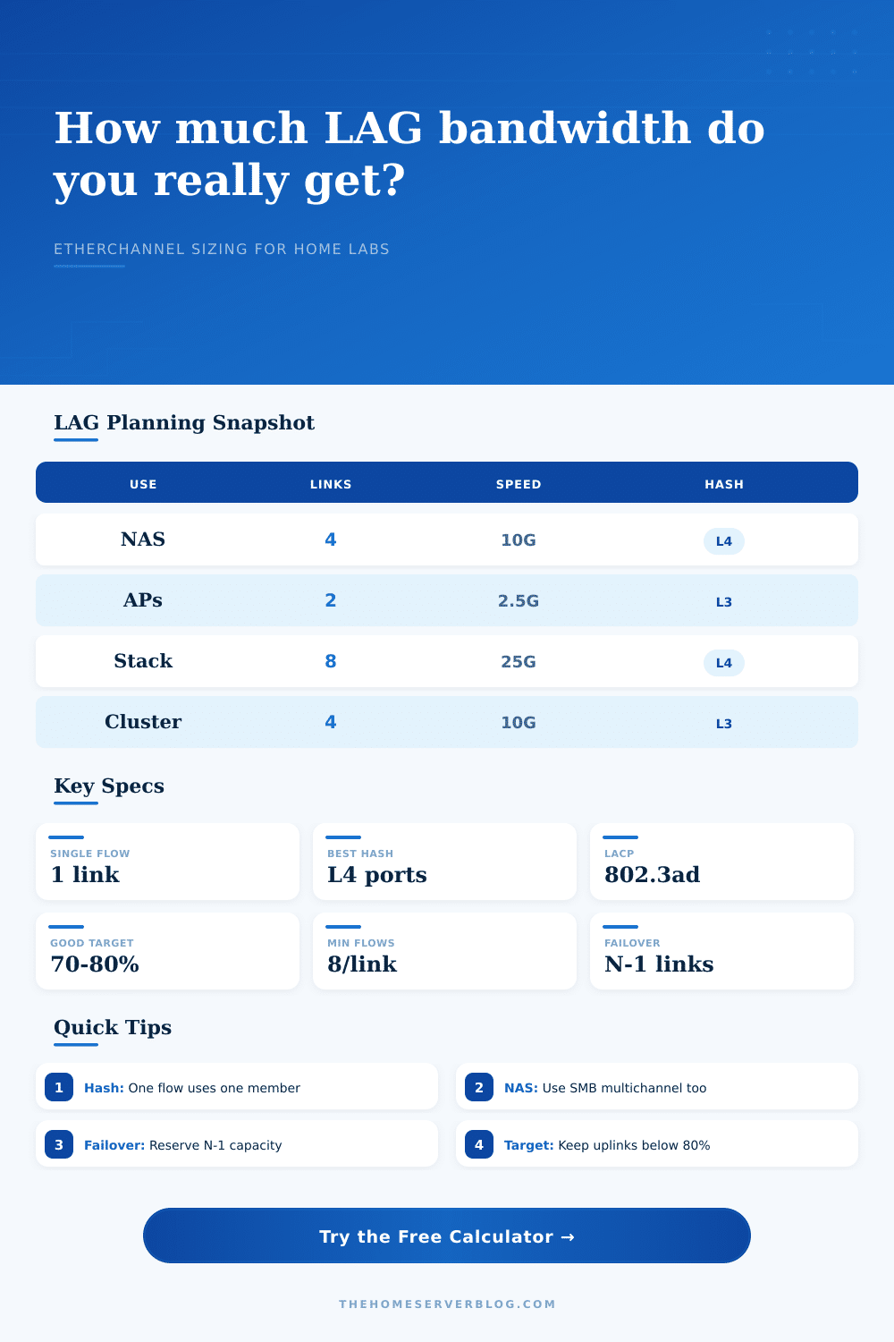
There are forty gigabits of raw throughput, which feels like an infinite amount when you see four switch port in front of you. Plug a Proxmox cluster or a NAS into that thing and expect maximum transfer speeds. Copy over a big file and it move along at a tenth of that: ten gigabits.
The hardware isn’t the problem. Traffic flowing through those links are the problem. EtherChannel doesn’t aggregate bandwidth for one huge conversation, but rather aggregates bandwidth for multiple conversations. That makes all the difference between a smooth and a frustrating network.
How EtherChannel Really Works
When you enter your preferred speeds and number of links, the calculator will do the rest. You don’t have to guess at conversions and coefficients. Concurrent flow count is the critical input. Flow is a unique TCP or UDP session identified by its source and destination addresses and ports. There’s one flow if one server back up to another. There are 50 flows if 50 users stream video.
Existing traffic is what gets bundled. You won’t find it slicing a single stream into several and sending each on a different wire. That would require knowing what’s in the stream before data arrived. Hashing methods makes this determination before they see the data, deciding which flow goes on which wire.
Layer 4 hashing examines both the port number and IP address when making its decision. It’s fine for most office traffic. There’s enough randomness in web surfing, emailing, and video calling to distribute traffic around nicely.
Not so with storage traffic. An iSCSI session, or even just copying a file over SMB, tends to hang around a tight range of ports. If you land on one link, it’ll max out while the other links twiddle their thumbs. Sure, you could throw another link into the bundle. But that one transfer can never be faster then one of those links. There’s a hard ceiling.
This is where failure planning becomes more than just a general idea; it’s something that can be practiced and used. Until you pull a switch port down, untie a cable, or some other way loosen a cable, a four link bundle seems fine. But suddenly you’re down to three links. The aggregate capacity drop by twenty-five percent instantly. And if you were already using eighty percent of the original capacity? That means you’re over subscribed. Queue builds up. Latency starts to spike. Even with all that apparent bandwidth, the network feels sluggish.
The calculator allows you to simulate the N minus one situation. It will show you what happens when hardware goes down.
As long as both switches understands each other, it doesn’t matter what protocol you use. LACP does this for a reason; it negotiates the bundle automatically. And it’s quick to detect when something goes wrong. PAgP is there because some old Cisco stuff won’t talk to anything except other Cisco. Static just works in a lab where nothing ever changes.
Hash distribution is really the variable here. Layer 2 hashing is great until your traffic collapses on fewer members if you’re using a router-on-a-stick to route traffic. All your traffic has the same router MAC. If you change the hashing to Layer 3 or Layer 4, it usually sorts out the imbalance based off the IP address behind the router.
Is the goal to max out each wire? No. The goal is to make the path as smooth as possible. To get the busiest window down to a 70-80% usage rate. Plan for room for backup jobs that run late and for bursts. And plan for how much more data there will inevitably be.
That’s why the table on the page has a reference for common setups, including core uplinks and Wi-Fi AP aggregation. Not just raw bandwidth but the safe planning target it spits out, that’s the number to tell you what the link can really handle before it chokes.
Part of network design is accounting. Part is art. Accounting is the part where you account for the overhead. Account for the encapsulation. Account for the VLAN tags. Account for the failure modes. Account for the flows. Art is the part where you realize that the numbers stop being useful at some point.
Let that terabyte-per-month transfer take an hour if you like. Don’t purchase additional fiber because of it. Invest in the links and hashing if you have to serve fifty VMs that need to talk to each other at the same time.
The calculator provides you with a baseline. Judgment fills in the gaps. On paper, you had forty gigabits. And now you know how many of those gigabits are actualy doing work for you.